论文解读GALA《SymmetricGraphConvolutionalAutoencoderforUnsupervisedGraphRepresentationLearning》

论文信息

　　Title：《Symmetric Graph Convolutional Autoencoder for Unsupervised Graph Representation Learning》
　　Authors：Jiwoong Park、Minsik Lee、H. Chang、Kyuewang Lee、J. Choi
　　Sources：2019 IEEE/CVF International Conference on Computer Vision (ICCV)
　　Paper：Download
　　Code：Download
　　Others：44 Citations, 44 References

---

Abstract

　　本文提出一个完全对称的自编码器，其中 解码器 基于 Laplacian sharpening  设计 ，编码器  基于 Laplacian smoothing 设计。此外还设计了一种基于  latent representation 和  affinity matrix  的代价函数。

---

1. Introduction

　　在机器学习和数据挖掘领域，使用图数据做以下研究：

• • node clustering 
  • dimensionality reduction 
  • social network analysis 
  • chemical property prediction of a molecular graph 
  • image segmentation 

　　卷积方法产生限制的原因：

• • Low computational efficiency due to eigendecomposition or singular value decomposition.
  • Only showing a shallow relationship between nodes.

 　　近年来，一个被称为几何深度学习（ geometric deep learning） 的新兴领域，将深度神经网络模型推广到 非欧几里得域 （ non-Euclidean domains），比如： meshes、 manifolds、 graphs。其中，利用自编码器框架寻找图的 geometrical structures 的深层潜在表示正越来越受到关注。

　　首先尝试的是   VGAE  它由一个  Graph Convolutional Network (GCN)  encoder   和一个  matrix outerproduct decoder  组成，如 Figure 1 (a) 所示。

　　作为  VGAE  的一种变体，ARVGA 采用了 VGAE 的  adversarial approach。然而 VGAE 和  ARVGA  重建   affinity matrix  $A$，而不是节点   feature matrix  $X $，因此，解码器部分不能是可学习的，故， graphical feature 不能在解码器部分中使用。 

　　之后，提出了  MGAE，它使用具有线性激活函数的堆叠单层图自动编码器和边缘化过程 如 Figure 1 (b)所示。但是， since the MGAE reconstructs the feature matrix of nodes without hidden layers, it cannot manipulate the dimension of the latent representation and performs a linear mapping.

　　　　

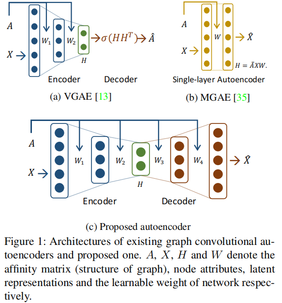
　　本文提出了一种新的图卷积自编码器框架，该框架具有对称的自编码器架构，并在编码和解码过程中同时使用图和节点属性，如 Figure 1(c)  所示 。

　　VGAE  的编码器可以解释为一种特殊形式的   Laplacian smoothing  ，它计算每个节点的新表示加权局部平均的邻居和本身。

　　本文使用切比雪夫多项式（Chebyshev polynomial）的形式表示拉普拉斯锐化以构造一个 Laplacian sharpening  的解码器。

　　本文贡献如下：

• • 提出了第一个完全对称的图卷积自编码器，它在整个编码-解码过程中同时利用了图的结构和节点属性。
  • 推导了一种新的数值稳定形式的防止神经网络数值不稳定的解码器。
  • 设计了一个计算高效的子空间聚类代价来同时寻找图像聚类任务的潜在表示和潜在亲和矩阵。

---

2. Preliminaries

2.1. Basic notations on graphs

• A graph is represented as  $\mathcal{G}=(\mathcal{V}, \mathcal{E}, A)$
• $\mathcal{V}$  denotes the node set with  $v_{i} \in \mathcal{V}$  and  $|\mathcal{V}|=n$.
• $\mathcal{E} $ denotes the edge set with  $\left(v_{i}, v_{j}\right) \in \mathcal{E} $.
• $A \in \mathbb{R}^{n \times n} $ denotes an affinity matrix which encodes pairwise affinities between nodes. 
• $D \in \mathbb{R}^{n \times n}$  denotes a degree matrix which is a diagonal matrix with  $D_{i i}=\sum_{j} A_{i j}$ .
• Unnormalized graph Laplacian  $\Delta$  is defined by  $\Delta=D-A$  .
• Symmetric graph Laplacian  $L$  is defined by  $L=I_{n}-D^{-\frac{1}{2}} A D^{-\frac{1}{2}}$ .
• Random walk graph Laplacian  $L_{r w}$ is defined by $L_{r w}=I_{n}-D^{-1} A$ 
• $I_{n} \in \mathbb{R}^{n \times n}  $  denotes an identity matrix.
• $\Delta$, $L$  and  $L_{r w}$ are positive semidefinite matrices.

2.2. Spectral convolution on graphs

　　可以发现 2.2 节的内容在《第三代GCN》已经将的很清楚了，所以下面不再详细展开介绍。

　　A spectral convolution on a graph is the multiplication of an input signal $x \in \mathbb{R}^{n}$ with a spectral filter $g_{\theta}=\operatorname{diag}(\theta)$ parameterized by the vector of Fourier coefficients $\theta \in \mathbb{R}^{n}$ as follows:

　　$g_{\theta} * x=U g_{\theta} U^{T} x\quad \quad \quad (1)$

　　where

• • $U$ is the matrix of eigenvectors of the symmetric graph Laplacian $L=U \Lambda U^{T}$ .
  • $U^{T} x$ is the graph Fourier transform of the input $x$ ,
  • $g_{\theta}$ is a function of the eigenvalues of $L$ .
  • $g_{\theta}(\Lambda)$ , where $\Lambda$ is the diagonal matrix of eigenvalues of $L$ .

　　一般图卷积带来的问题：this operation is inappropriate for large-scale graphs since it requires an eigendecomposition to obtain the eigenvalues and eigenvectors of $L$ .

　　解决办法：the spectral filter $g_{\theta}(\Lambda)$ was approximated by $K^{t h}$ order Chebyshev polynomials in previous works . By doing so, the spectral convolution on the graph can be approximated as

　　　　$g_{\theta} * x \approx U \sum\limits _{k=0}^{K} \theta_{k}^{\prime} T_{k}(\tilde{\Lambda}) U^{T} x=\sum\limits _{k=0}^{K} \theta_{k}^{\prime} T_{k}(\tilde{L}) x\quad \quad \quad (2)$

　　where 

• • $T_{k}(\cdot)$ denote the Chebyshev polynomials .
  • $\theta^{\prime}$ denote a vector of the Chebyshev coefficients.
  • $\tilde{\Lambda}$ is $\frac{2}{\lambda_{\max }} \Lambda-I_{n}$.
  • $\lambda_{\max }$ denotes the largest eigenvalue of $L$.
  • $\tilde{L}$ is $U \tilde{\Lambda} U^{T}=\frac{2}{\lambda_{\max }} L-I_{n} $. 

　　In the GCN , the Chebyshev approximation model was simplified by setting $K=1$, $\lambda_{\max } \approx 2$ and $\theta=\theta_{0}^{\prime}= -\theta_{1}^{\prime}$ . This makes the spectral convolution simplified as follows:

　　　　$g_{\theta} * x \approx \theta\left(I_{n}+D^{-\frac{1}{2}} A D^{-\frac{1}{2}}\right) x  \quad \quad \quad (3)$

　　However, repeated application of $I_{n}+D^{-\frac{1}{2}} A D^{-\frac{1}{2}}$ can cause numerical instabilities in neural networks since the spectral radius of $I_{n}+D^{-\frac{1}{2}} A D^{-\frac{1}{2}}$ is $2$ , and the Chebyshev polynomials form an orthonormal basis when its spectral radius is $1$ . To circumvent this issue, the GCN uses renormalization trick:

　　　　$I_{n}+D^{-\frac{1}{2}} A D^{-\frac{1}{2}} \rightarrow \tilde{D}^{-\frac{1}{2}} \tilde{A} \tilde{D}^{-\frac{1}{2}}  \quad \quad \quad (4)$

　　where $\tilde{A}=A+I_{n}$ and $\tilde{D}_{i i}=\sum_{j} \tilde{A}_{i j}$ . Since adding selfloop on nodes to an affinity matrix cannot affect the spectral radius of the corresponding graph Laplacian matrix , this renormalization trick can provide a numerically stable form of $I_{n}+D^{-\frac{1}{2}} A D^{-\frac{1}{2}}$ while maintaining the meaning of each elements as follows:

　　　　$\left(I_{n}+D^{-\frac{1}{2}} A D^{-\frac{1}{2}}\right)_{i j}=\left\{\begin{array}{ll}1 & i=j \\A_{i j} / \sqrt{D_{i i} D_{j j}} & i \neq j\end{array}\right.\quad \quad \quad (5)$

　　　　$\left(\tilde{D}^{-\frac{1}{2}} \tilde{A} \tilde{D}^{-\frac{1}{2}}\right)_{i j}=\left\{\begin{array}{ll}1 /\left(D_{i i}+1\right) & i=j \\A_{i j} / \sqrt{\left(D_{i i}+1\right)\left(D_{j j}+1\right)} & i \neq j\end{array}\right.\quad \quad \quad (6)$

　　Finally, the forward-path of the GCN can be expressed by

　　　　$H^{(m+1)}=\xi\left(\tilde{D}^{-\frac{1}{2}} \tilde{A} \tilde{D}^{-\frac{1}{2}} H^{(m)} \Theta^{(m)}\right)\quad \quad \quad (7)$

　　where $H^{(m)}$  is the activation matrix in the $m^{t h}$  layer and $H^{(0)}$  is the input nodes' feature matrix $X $. $\xi(\cdot)$  is a nonlinear activation function like $\operatorname{ReLU}(\cdot)=\max (0, \cdot) $, and $\Theta^{(m)}$  is a trainable weight matrix. The GCN presents a computationally efficient convolutional process (given the assumption that $\tilde{A}$  is sparse) and achieves an improved accuracy over the state-of-the-art methods in semi-supervised node classification task by using features of nodes and geometric structure of graph simultaneously.

2.3. Laplacian smoothing

　　 Li et al. show that GCN is a special form of Laplacian smoothing.

　　Laplacian smoothing equation:

　　　　$x_{i}^{(m+1)}=(1-\gamma) x_{i}^{(m)}+\gamma \sum\limits_{j} \frac{\tilde{A}_{i j}}{\tilde{D}_{i i}} x_{j}^{(m)}\quad \quad \quad (8)$

 　　Where:

• • $\tilde{A}=A+I_{n}$.
  • $\tilde{D}=D+I_{n}$.
  • $x_{i}^{(m+1)}$ is the new representation of $x_{i}^{(m)}$.
  • $\gamma (0<\gamma \leq 1)$ is a regularization parameter which controls the importance between itself and its neighbors. 

　　Rewrite the above equation in a matrix form as follows:

　　　　$\begin{aligned}X^{(m+1)} &=(1-\gamma) X^{(m)}+\gamma \tilde{D}^{-1} \tilde{A} X^{(m)} \\&=X^{(m)}-\gamma\left(I_{n}-\tilde{D}^{-1} \tilde{A}\right) X^{(m)} \\&=X^{(m)}-\gamma \tilde{L}_{r w} X^{(m)}\end{aligned}\quad \quad \quad (9)$

Tips:

　　Random walk normalized Laplacian 

 　　　　$L^{r w}=D^{-1} L=I-D^{-1} A$

　　Symmetric normalized Laplacian

　　　　$L^{\text {sys }}=D^{-1 / 2} L D^{-1 / 2}=I-D^{-1 / 2} A D^{-1 / 2}$

 　　We set  $\gamma=1$  and replace $\tilde{L}_{r w}$  with  $\tilde{L}$ , then Eq. (9) is changed into 

　　　　$X^{(m+1)}=\tilde{D}^{-\frac{1}{2}} \tilde{A} \tilde{D}^{-\frac{1}{2}} X^{(m)}$ 

　　This equation is the same as the renormalized version of spectral convolution in Eq. (7).

---

3 The proposed method

　　Our mode is GALA (Graph convolutional Autoencoder using Laplacian smoothing and sharpening).

　　In GALA, there are  $M$  layers in total, from the first to $\frac{M}{2}$  th layers for the encoder and from the  $\left(\frac{M}{2}+1\right)$ th to  $M$  th layers for the decoder where  $M$  is an even number.

• The encoder part of GALA is designed to perform the computationally efficient spectral convolution on the graph with a numerically stable form of Laplacian smoothing in the Eq. (7) .
• Its decoder part is designed to be a special form of Laplacian sharpening . By this decoder part, GALA reconstructs the feature matrix of nodes directly, instead of yielding an affinity matrix as in the existing VGAE-related algorithms whose decoder parts are incomplete.

3.1 Laplacian sharpening

　　The encoder performs Laplacian smoothing that makes the latent representation of each node similar to those of its neighboring nodes.

　　Laplacian sharpening is a process that makes the reconstructed feature of each node farther away from the centroid of its neighbors.

　　Laplacian sharpening equation:

 　　　　$x_{i}^{(m+1)}=(1+\gamma) x_{i}^{(m)}-\gamma \sum\limits _{j} \frac{A_{i j}}{D_{i i}} x_{j}^{(m)}\quad \quad \quad (10)$

 　　Where:

• • $x_{i}^{(m+1)}$ is the new representation of $x_{i}^{(m)}$.
  • $\gamma (0<\gamma \leq 1)$ is a regularization parameter which controls the importance between itself and its neighbors. 

　　 The matrix form of Eq. (10) :

　　　　$\begin{aligned}X^{(m+1)} &=(1+\gamma) X^{(m)}-\gamma D^{-1} A X^{(m)} \\&=X^{(m)}+\gamma\left(I_{n}-D^{-1} A\right) X^{(m)} \\&=X^{(m)}+\gamma L_{r w} X^{(m)}\end{aligned}\quad \quad \quad (11)$

　　We set  $\gamma=1$  and replace $\tilde{L}_{r w}$  with  $\tilde{L}$ , then Eq. (10) is changed into 

 　　　　$X^{(m+1)}=(2 I_{n}-D^{-\frac{1}{2}} A D^{-\frac{1}{2}})X^{(m)}$

　　We express Laplacian sharpening in the form of Chebyshev polynomial  and simplify it with 

• • $K=1$　　
  • $\lambda_{\max } \approx 2$
  • $\theta=\frac{1}{2} \theta_{0}^{\prime}=\theta_{1}^{\prime}$

　　Then, a decoder layer can be expressed by

　　　　$H^{(m+1)}=\xi\left(\left(2 I_{n}-D^{-\frac{1}{2}} A D^{-\frac{1}{2}}\right) H^{(m)} \Theta^{(m)}\right)\quad \quad \quad (12)$

　　Where:

• • $H^{(m)}$  is the matrix of the activation in the  $m^{t h}$  layer, 
  • $2 I_{n}-D^{-\frac{1}{2}} A D^{-\frac{1}{2}}$  is a special form of Laplacian sharpening, 
  • $\xi(\cdot)$  is the nonlinear activation function like  $\operatorname{ReLU}(\cdot)   =\max (0, \cdot)$ ,
  • $\Theta^{(m)}$  is a trainable weight matrix.

　　The spectral radius of  $2 I_{n}-D^{-\frac{1}{2}} A D^{-\frac{1}{2}}$  is 3 , repeated application of this operator can be numerically instable. 

       方阵的谱半径

　　若 $\boldsymbol{A}=\left(a_{i j}\right)$ 是复数域上的 $\mathrm{n} $ 阶方阵，又 $\lambda_{1}, \lambda_{2}, \ldots, \lambda_{n}$ 是 $A$ 的全部特征值，则

　　　　$\rho(\boldsymbol{A})= \underset{1 \leq i \leq n}{max}  |\lambda_{i}|$

　　From previous articles,we know that 

　　　　$D^{-\frac{1}{2}} A D^{-\frac{1}{2}}$ range  $[ -1,1]$

 　　So we need to find a  numerically stable form of Laplacian sharpening.

3.2 Numerically stable Laplacian sharpening

　　To find a new representation of Laplacian sharpening whose spectral radius is $1$ .

　　A signed graph is denoted by  $\Gamma=(\mathcal{V}, \mathcal{E}, \hat{A})$  which is induced from the unsigned graph  $\mathcal{G}=(\mathcal{V}, \mathcal{E}, A)$ .

　　Each element in  $\hat{A}$  has the same absolute value with  $A$ , but its sign is changed into minus or keeps plus.

　　The degree matrix $\hat{D}$ can be defined as $\hat{D}_{i i}=\sum\limits _{j}\left|\hat{A}_{i j}\right|$ .

　　Thus,we can construct

• • unnormalized graph Laplacian  $\hat{\Delta}=\hat{D}-\hat{A}$.
  • symmetric graph Laplacian  $\hat{L}=I_{n}-\hat{D}^{-\frac{1}{2}} \hat{A} \hat{D}^{-\frac{1}{2}}$  of the signed graph.

　　The range of the eigenvalue of  $\hat{L}$  is  $[0,2]$ , thus the spectral radius of  $\hat{D}^{-\frac{1}{2}} \hat{A} \hat{D}^{-\frac{1}{2}}$  is $1$ for any choice of  $\hat{A}$ . 

　　 Using this result, instead of Eq. (12):

　　　　$H^{(m+1)}=\xi\left(\hat{D}^{-\frac{1}{2}} \hat{A} \hat{D}^{-\frac{1}{2}} H^{(m)} \Theta^{(m)}\right)\quad \quad \quad (13)$

　　Where:

• • $\hat{A}=2 I_{n}-A$　　
  • $\hat{D}=2 I_{n}+D$

　　$\hat{D}^{-\frac{1}{2}} \hat{A} \hat{D}^{-\frac{1}{2}}$ 计算方式如下：

　　　　$\left(\hat{D}^{-\frac{1}{2}} \hat{A} \hat{D}^{-\frac{1}{2}}\right)_{i j}=\left\{\begin{array}{ll}2 /\left(D_{i i}+2\right) & i=j \\-A_{i j} / \sqrt{\left(D_{i i}+2\right)\left(D_{j j}+2\right)} & i \neq j\end{array}\right.\quad \quad \quad (14)$

　　Which has the same meaning with the original one given by

　　　　$\left(2 I_{n}-D^{-\frac{1}{2}} A D^{-\frac{1}{2}}\right)_{i j}=\left\{\begin{array}{ll}2 & i=j \\-A_{i j} / \sqrt{D_{i i} D_{j j}} & i \neq j\end{array}\right.\quad \quad \quad (15)$

　　目的：

• • 将谱半径变成 $1$。
  • $\hat{D}^{-\frac{1}{2}} \hat{A} \hat{D}^{-\frac{1}{2}}$  保留了和  $2 I_{n}-D^{-\frac{1}{2}} A D^{-\frac{1}{2}}$  的性质。

 　　Sumary, the numerically stable decoder layer of GALA is given as

　　　　$H^{(m+1)}=\xi\left(\hat{D}^{-\frac{1}{2}} \hat{A} \hat{D}^{-\frac{1}{2}} H^{(m)} \Theta^{(m)}\right),\left(m=\frac{M}{2}, \ldots, M-1\right)\quad \quad \quad (16)$

　　Where

• • $\hat{A}=2 I_{n}-A$　　
  • $\hat{D}=2 I_{n}+D$

 　　 The encoder layer of GALA is given as

　　　　$H^{(m+1)}=\xi\left(\tilde{D}^{-\frac{1}{2}} \tilde{A} \tilde{D}^{-\frac{1}{2}} H^{(m)} \Theta^{(m)}\right),\left(m=0, \ldots, \frac{M}{2}-1\right)\quad \quad \quad (17)$

　　Where

• • $\tilde{A}=I_{n}+A$
  • $\tilde{D}=I_{n}+D$

　　 Both encoder and decoder propagation functions, Eqs. (16) and (17), are both $\mathcal{O}(m p c)$.

• • $m$ is the cardinality of edges in the graph.
  • $p$ is the feature dimension of the previous layer.
  • $c$ is the feature dimension of the current layer.

　　In Table 1, we show the reason why the Laplacian smoothing is not appropriate to the decoder and the necessity of numerically stable Laplacian sharpening by node clustering experiments.

　　　　

• Laplacian smoothing decoder (Eq. 7) shows the lowest performances, since Laplacian smoothing which makes the representation of each node similar to those of its neighboring nodes conflicts with the purpose of reconstruction cost.
• A numerically instable form of Laplacian sharpening decoder (Eq. 12) shows higher performance compared to smoothing decoder because the role of Laplacian sharpening coincide with reconstructing the node feature.
• The performance of proposed numerically stable Laplacian sharpening decoder (Eq. 16) significantly higher than others, since it solves instability issue of neural network while maintaining the meaning of original Laplacian sharpening.

　　The basic cost function of GALA is given by

 　　　　$\min _{\bar{X}} \frac{1}{2}\|X-\bar{X}\|_{F}^{2}\quad \quad \quad (18)$

 　　Where

• • $\bar{X}$  is the reconstructed feature matrix of nodes.
  • the column of  $\bar{X}$  corresponds to the output of the decoder for an input feature of a node.
  • $\|\cdot\|_{F}$  denotes the Frobenius norm.

3.3. Subspace clustering cost for image clustering

　　For image clustering tasks,we add  an element of subspace clustering to the proposed method.

　　　　$\underset{\bar{X}, H, A_{H}}{min} \frac{1}{2}\|X-\bar{X}\|_{F}^{2}+\frac{\lambda}{2}\left\|H-H A_{H}\right\|_{F}^{2}+\frac{\mu}{2}\left\|A_{H}\right\|_{F}^{2}\quad \quad \quad (19)$

 　　Where

• • $H \in \mathbb{R}^{k \times n}$  denotes the latent representations (i.e., the output of the encoder).
  • $A_{H} \in \mathbb{R}^{n \times n}$  denotes the affinity matrix which is a new latent variable for subspace clustering,
  • $ \lambda$, $\mu$  are the regularization parameters.

　　The second term of Eq. (19) aims at the self-expressive model of subspace clustering and the third term of Eq. (19) is for regularizing  $A_{H}$ .

　　If we only consider minimizing  $A_{H}$ , the problem becomes:

 　　　　$\underset{A_{H}}{min}    \frac{\lambda}{2}\left\|H-H A_{H}\right\|_{F}^{2}+\frac{\mu}{2}\left\|A_{H}\right\|_{F}^{2}\quad \quad \quad (20)$

　　We can easily obtain the analytic solution

　　　　$A_{H}^{*}=(H^{T} H+\frac{\mu}{\lambda} I_{n})^{-1} H^{T} H $

　　By using this analytic solution and singular value decomposition, we derive a computationally efficient subspace clustering cost function as follows :

　　　　$\underset{\bar{X}, H}{min}  \frac{1}{2}\|X-\bar{X}\|_{F}^{2}+\frac{\mu \lambda}{2} \operatorname{tr}\left(\left(\mu I_{k}+\lambda H H^{T}\right)^{-1} H H^{T}\right)\quad \quad \quad (21)$

　　Some benefits are it can reduce the computational burden significantly.

• • The above problem can be solved by  $k \times k$  matrix inversion instead of  $n \times n$ matrix inversion.  from  $\mathcal{O}\left(n^{3}\right)$  to  $\mathcal{O}\left(k^{3}\right)$ .
  • $k$ is the dimension of latent representation.

3.4. Training

• We train GALA to minimize Eq. (18) by using the ADAM algorithm.
• We train GALA deterministically by using the full batch in each training epoch and stop when the cost is converged.
• We set the learning rate to $1.0 × 10^{-4}$ for training and train GALA in an unsupervised way without any cluster labels.

　　For image clustering tasks,we add the subspace clustering cost is added to reconstruction cost.

• • First, in the pre-training stage, the training method is the same as that of minimizing Eq. (18).
  • After pre-training, we fine-tune GALA to minimize Eq. (21) using ADAM.

　　After the training process are over, we construct  $k$  nearest neighborhood graph using attained latent representations  $H^{*}$ . Then we perform spectral clustering and get the clustering performance.

　　In the case of image clustering, after all training processes are over, we construct the optimal affinity matrix  $A_{H}^{*}$  noted in the previous subsection by using the attained latent representation matrix  $H^{*}$  from GALA. Then we perform spectral clustering on the affinity matrix and get the optimal clustering with respect to our cost function.

---

4. Experiments

4.1. Datasets

　　Four network datasets

• • Cora
  • Citeseer
  • Wik
  • Pubmed

　　Every network dataset has the feature matrix $X$ and the affinity matrix $A$ .

　　Three image datasets 

• • COIL20
  • YALE
  • MNIST

　　Every image dataset has the feature matrix $X$ only.　　

　　Task：

• • Node clustering.
  • Link prediction tasks.

4.2. Experimental settings

　　Three metrics:

• • accuracy (ACC)
  • normalized mutual information (NMI)
  • adjusted rand index (ARI)

　　For average in 50 times.

4.3. Comparing methods

• Using features only.
  • Kmeans
• Using network structures only.
  • Spectral
  • Big-Clam
  • DeepWalk
  • GraEnc
  • DNGR
• Using both
  
  • Circles
  • RTM
  • RMSC
  • TADW
• Using both with spectral convolution on graphs
  • GAE
  • VGAE
  • MGAE
  • ARGA
  • ARVGA

　　

4.4. Node clustering results

　　The experimental results of node clustering are presented in Table 2.

　　　　

• For every dataset, the methods which use features and network structures simultaneously show better performance than the methods which use only one of them.
• Use both features and network structures, algorithms with neural network models which exploit spectral convolution on graphs present outstanding performance since they can learn deeper relationships between nodes than the methods which do not use spectral convolution on graphs.
• GALA shows superior performance to other methods.
• MGAE, which is the state-of-the-art graph convolutional autoencoder algorithm, by about 6.15%, 6.56% and 8.68% on ACC, NMI and ARI.
• The better performance of GALA comes from the better decoder design based on the numerically stable form of Laplacian sharpening both and full utilizing of graph structure and node attributes in the whole autoencoder framework.

　　We conduct another node clustering experiment on a large network dataset (Pubmed), and the results are reported in Table 5.

　　　　

• GALA outperforms every baselines and state-of-the-art graph convolution algorithms.

4.5. Image clustering results

　　The experimental results of image clustering are presented in Table 4.

　　 We report both GALA’s performance of reconstruction cost only case and the subspace clustering cost added case (GALA+SCC).

　　

• GALA outperforms several baselines and the state-of-the-art graph convolution algorithms for most of the cases.
• The proposed subspace clustering cost term contributes to improve the performance of the image clustering.

4.6. Ablation studies

　　 We validate the effectiveness of the proposed stable decoder and the subspace clustering cost by image clustering experiments on the three image datasets (COIL20, YALE and MNIST).

　　 There are four configurations as shown in Table 6.

　　　　

• The numerically stable form of Laplacian sharpening and subspace clustering cost are helpful to find the latent representations.
• Stable decoder with the reconstruction cost only outperforms the state-of-the-art algorithms in most cases

4.7. Link prediction results

　　We provide some results on link prediction task on Citeseer dataset.

　　For link prediction task, we minimized the below cost function that added link prediction cost of GAE to the reconstruction cost

 　　　　$\underset{\bar{X}, H}{min} \frac{1}{2}\|X-\bar{X}\|_{F}^{2}+\gamma \mathbb{E}_{H}[\log p(\hat{A} \mid H)]$

　　where 

• • $H$  is the latent representation, 
  • $\hat{A}=\operatorname{sigmoid}\left(H H^{T}\right)$  is the reconstructed affinity matrix and 
  • $\gamma$  is the regularization parameter.

　　The results are shown in Table 7

　　　　

• Our model outperforms the compared methods in terms of the link prediction task as well as the node clustering task.

4.8. Visualization

• The encoder makes the feature of each node becomes similar with its neighbors.
• The decoder makes the features of each node distinguishable with its neighbors using the geometrical structure of the graphs.

　　We visualize the distribution of learned latent representations and the input features of each node in two-dimensional space using t-SNE [23] as shown in Figure 3.

　　　　

• From the visualization, we can see that GALA is wellclustering the data according to their corresponding labels even though GALA performs in an unsupervised manner.
• We can see through the red dotted line in embedding results of the latent representation on YALE that GALA embeds the representation of nodes better than the compared methods by minimizing inter-cluster affinity and maximizing intra-cluster affinity

---

5. Conclusions

• We designed a symmetric graph convolutional autoencoder architecture where the encoder performs Laplacian smoothing while the decoder performs Laplacian sharpening.
• To prevent numerical instabilities, we designed a new representation of Laplacian sharpening with spectral radius one by incorporating the concept of the signed graph.
• To enhance the performance of image clustering tasks, we added a subspace clustering cost term to the reconstruction cost of the autoencoder.