Catboost等模型]--模型融合：stacking、blending

1.赛题简介

赛题以金融风控中的个人信贷为背景，要求选手根据贷款申请人的数据信息预测其是否有违约的可能，以此判断是否通过此项贷款，这是一个典型的分类问题。通过这道赛题来引导大家了解金融风控中的一些业务背景，解决实际问题，帮助竞赛新人进行自我练习、自我提高。

赛题以预测金融风险为任务，数据集报名后可见并可下载，该数据来自某信贷平台的贷款记录，总数据量超过120w，包含47列变量信息，其中15列为匿名变量。为了保证比赛的公平性，将会从中抽取80万条作为训练集，20万条作为测试集A，20万条作为测试集B，同时会对employmentTitle、purpose、postCode和title等信息进行脱敏。

比赛地址：https://tianchi.aliyun.com/competition/entrance/531830/introduction

项目链接以及码源见文末

1.1数据介绍

赛题以预测用户贷款是否违约为任务，数据集报名后可见并可下载，该数据来自某信贷平台的贷款记录，总数据量超过120w，包含47列变量信息，其中15列为匿名变量。为了保证比赛的公平性，将会从中抽取80万条作为训练集，20万条作为测试集A，20万条作为测试集B，同时会对employmentTitle、purpose、postCode和title等信息进行脱敏。

一般而言，对于数据在比赛界面都有对应的数据概况介绍（匿名特征除外），说明列的性质特征。了解列的性质会有助于我们对于数据的理解和后续分析。 Tip:匿名特征，就是未告知数据列所属的性质的特征列。

train.csv

id 为贷款清单分配的唯一信用证标识
loanAmnt 贷款金额
term 贷款期限（year）
interestRate 贷款利率
installment 分期付款金额
grade 贷款等级
subGrade 贷款等级之子级
employmentTitle 就业职称
employmentLength 就业年限（年）
homeOwnership 借款人在登记时提供的房屋所有权状况
annualIncome 年收入
verificationStatus 验证状态
issueDate 贷款发放的月份
purpose 借款人在贷款申请时的贷款用途类别
postCode 借款人在贷款申请中提供的邮政编码的前3位数字
regionCode 地区编码
dti 债务收入比
delinquency_2years 借款人过去2年信用档案中逾期30天以上的违约事件数
ficoRangeLow 借款人在贷款发放时的fico所属的下限范围
ficoRangeHigh 借款人在贷款发放时的fico所属的上限范围
openAcc 借款人信用档案中未结信用额度的数量
pubRec 贬损公共记录的数量
pubRecBankruptcies 公开记录清除的数量
revolBal 信贷周转余额合计
revolUtil 循环额度利用率，或借款人使用的相对于所有可用循环信贷的信贷金额
totalAcc 借款人信用档案中当前的信用额度总数
initialListStatus 贷款的初始列表状态
applicationType 表明贷款是个人申请还是与两个共同借款人的联合申请
earliesCreditLine 借款人最早报告的信用额度开立的月份
title 借款人提供的贷款名称
policyCode 公开可用的策略_代码=1新产品不公开可用的策略_代码=2
n系列匿名特征匿名特征n0-n14，为一些贷款人行为计数特征的处理

1.2预测指标

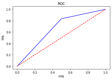
竞赛采用AUC作为评价指标。AUC（Area Under Curve）被定义为 ROC曲线下与坐标轴围成的面积。

1.2.1 分类算法常见的评估指标如下：

1、混淆矩阵（Confuse Matrix）

（1）若一个实例是正类，并且被预测为正类，即为真正类TP(True Positive )
（2）若一个实例是正类，但是被预测为负类，即为假负类FN(False Negative )
（3）若一个实例是负类，但是被预测为正类，即为假正类FP(False Positive )
（4）若一个实例是负类，并且被预测为负类，即为真负类TN(True Negative )

2、准确率（Accuracy）
准确率是常用的一个评价指标，但是不适合样本不均衡的情况。
$Accuracy = \frac{TP + TN}{TP + TN + FP + FN}$

3、精确率（Precision）
又称查准率，正确预测为正样本（TP）占预测为正样本(TP+FP)的百分比。
$Precision = \frac{TP}{TP + FP}$

4、召回率（Recall）
又称为查全率，正确预测为正样本（TP）占正样本(TP+FN)的百分比。
$Recall = \frac{TP}{TP + FN}$

5、F1 Score
精确率和召回率是相互影响的，精确率升高则召回率下降，召回率升高则精确率下降，如果需要兼顾二者，就需要精确率、召回率的结合F1 Score。
$F1-Score = \frac{2}{\frac{1}{Precision} + \frac{1}{Recall}}$

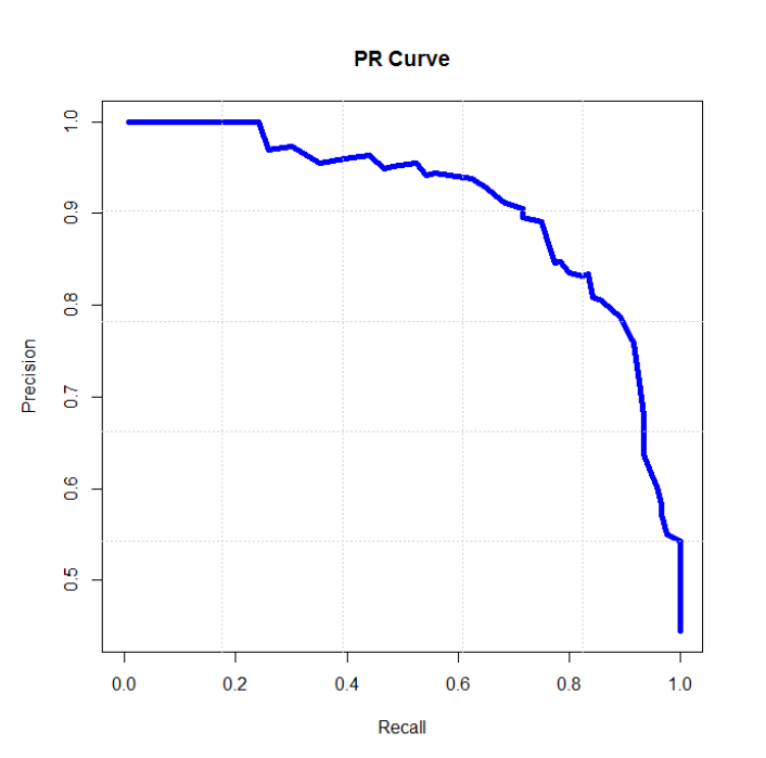
6、P-R曲线（Precision-Recall Curve）
P-R曲线是描述精确率和召回率变化的曲线

7、ROC（Receiver Operating Characteristic）

ROC空间将假正例率（FPR）定义为 X 轴，真正例率（TPR）定义为 Y 轴。

TPR：在所有实际为正例的样本中，被正确地判断为正例之比率。
$TPR = \frac{TP}{TP + FN}$
FPR：在所有实际为负例的样本中，被错误地判断为正例之比率。
$FPR = \frac{FP}{FP + TN}$

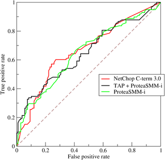
8、AUC(Area Under Curve)
AUC（Area Under Curve）被定义为 ROC曲线下与坐标轴围成的面积，显然这个面积的数值不会大于1。又由于ROC曲线一般都处于y=x这条直线的上方，所以AUC的取值范围在0.5和1之间。AUC越接近1.0，检测方法真实性越高;等于0.5时，则真实性最低，无应用价值。

1.2.2 对于金融风控预测类常见的评估指标如下:

1、KS(Kolmogorov-Smirnov)
KS统计量由两位苏联数学家A.N. Kolmogorov和N.V. Smirnov提出。在风控中，KS常用于评估模型区分度。区分度越大，说明模型的风险排序能力（ranking ability）越强。
K-S曲线与ROC曲线类似，不同在于

ROC曲线将真正例率和假正例率作为横纵轴
K-S曲线将真正例率和假正例率都作为纵轴，横轴则由选定的阈值来充当。
公式如下：
$KS=max(TPR-FPR)$
KS不同代表的不同情况，一般情况KS值越大，模型的区分能力越强，但是也不是越大模型效果就越好，如果KS过大，模型可能存在异常，所以当KS值过高可能需要检查模型是否过拟合。以下为KS值对应的模型情况，但此对应不是唯一的，只代表大致趋势。

KS（%）	好坏区分能力
20以下	不建议采用
20-40	较好
41-50	良好
51-60	很强
61-75	非常强
75以上	过于高，疑似存在问题

2、ROC

3、AUC

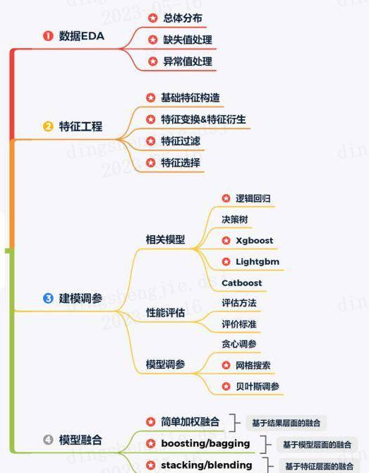
1.3 项目流程介绍

1.4 代码示例

本部分为对于数据读取和指标评价的示例。

1.4.1 数据读取pandas

import pandas as pd

train = pd.read_csv('train.csv')
testA = pd.read_csv('testA.csv')

print('Train data shape:',train.shape)
print('TestA data shape:',testA.shape)

Train data shape: (800000, 47)
TestA data shape: (200000, 48)

train.head()

1.4.2 分类指标评价计算示例

## 混淆矩阵
import numpy as np
from sklearn.metrics import confusion_matrix
y_pred = [0, 1, 0, 1]
y_true = [0, 1, 1, 0]
print('混淆矩阵:\n',confusion_matrix(y_true, y_pred))

混淆矩阵:
 [[1 1]
 [1 1]]

## accuracy
from sklearn.metrics import accuracy_score
y_pred = [0, 1, 0, 1]
y_true = [0, 1, 1, 0]
print('ACC:',accuracy_score(y_true, y_pred))

ACC: 0.5

## Precision,Recall,F1-score
from sklearn import metrics
y_pred = [0, 1, 0, 1]
y_true = [0, 1, 1, 0]
print('Precision',metrics.precision_score(y_true, y_pred))
print('Recall',metrics.recall_score(y_true, y_pred))
print('F1-score:',metrics.f1_score(y_true, y_pred))

Precision 0.5
Recall 0.5
F1-score: 0.5

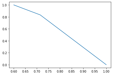
## P-R曲线
import matplotlib.pyplot as plt
from sklearn.metrics import precision_recall_curve
y_pred = [0, 1, 1, 0, 1, 1, 0, 1, 1, 1]
y_true = [0, 1, 1, 0, 1, 0, 1, 1, 0, 1]
precision, recall, thresholds = precision_recall_curve(y_true, y_pred)
plt.plot(precision, recall)

[<matplotlib.lines.Line2D at 0x2170d0d6108>]

## ROC曲线
from sklearn.metrics import roc_curve
y_pred = [0, 1, 1, 0, 1, 1, 0, 1, 1, 1]
y_true = [0, 1, 1, 0, 1, 0, 1, 1, 0, 1]
FPR,TPR,thresholds=roc_curve(y_true, y_pred)
plt.title('ROC')
plt.plot(FPR, TPR,'b')
plt.plot([0,1],[0,1],'r--')
plt.ylabel('TPR')
plt.xlabel('FPR')

Text(0.5, 0, 'FPR')

## AUC
import numpy as np
from sklearn.metrics import roc_auc_score
y_true = np.array([0, 0, 1, 1])
y_scores = np.array([0.1, 0.4, 0.35, 0.8])
print('AUC socre:',roc_auc_score(y_true, y_scores))

AUC socre: 0.75

## KS值 在实际操作时往往使用ROC曲线配合求出KS值
from sklearn.metrics import roc_curve
y_pred = [0, 1, 1, 0, 1, 1, 0, 1, 1, 1]
y_true = [0, 1, 1, 0, 1, 0, 1, 1, 1, 1]
FPR,TPR,thresholds=roc_curve(y_true, y_pred)
KS=abs(FPR-TPR).max()
print('KS值：',KS)

KS值： 0.5238095238095237

1.5 拓展知识——评分卡

评分卡是一张拥有分数刻度会让相应阈值的表。信用评分卡是用于用户信用的一张刻度表。以下代码是一个非标准评分卡的代码流程，用于刻画用户的信用评分。评分卡是金融风控中常用的一种对于用户信用进行刻画的手段哦！

#评分卡 不是标准评分卡
def Score(prob,P0=600,PDO=20,badrate=None,goodrate=None):
    P0 = P0
    PDO = PDO
    theta0 = badrate/goodrate
    B = PDO/np.log(2)
    A = P0 + B*np.log(2*theta0)
    score = A-B*np.log(prob/(1-prob))
    return score

2.数据探索性分析

目的：

1.EDA价值主要在于熟悉了解整个数据集的基本情况（缺失值，异常值），对数据集进行验证是否可以进行接下来的机器学习或者深度学习建模.
2.了解变量间的相互关系、变量与预测值之间的存在关系。
3.为特征工程做准备

2.1 代码示例

2.1.1 导入数据分析及可视化过程需要的库

import pandas as pd
import numpy as np
import matplotlib.pyplot as plt
import seaborn as sns
import datetime
import warnings
warnings.filterwarnings('ignore')

/Users/exudingtao/opt/anaconda3/lib/python3.7/site-packages/statsmodels/tools/_testing.py:19: FutureWarning: pandas.util.testing is deprecated. Use the functions in the public API at pandas.testing instead.
  import pandas.util.testing as tm

以上库都是pip install 安装就好，如果本机有python2,python3两个python环境傻傻分不清哪个的话,可以pip3 install 。或者直接在notebook中'!pip3 install ****'安装。

2.1.2 读取文件

data_train = pd.read_csv('./train.csv')

data_test_a = pd.read_csv('./testA.csv')

读取文件的拓展知识

pandas读取数据时相对路径载入报错时，尝试使用os.getcwd()查看当前工作目录。
TSV与CSV的区别：
- 从名称上即可知道，TSV是用制表符（Tab,'\t'）作为字段值的分隔符；CSV是用半角逗号（','）作为字段值的分隔符；
- Python对TSV文件的支持：
  Python的csv模块准确的讲应该叫做dsv模块，因为它实际上是支持范式的分隔符分隔值文件（DSV，delimiter-separated values）的。
  delimiter参数值默认为半角逗号，即默认将被处理文件视为CSV。当delimiter='\t'时，被处理文件就是TSV。
读取文件的部分（适用于文件特别大的场景）
- 通过nrows参数，来设置读取文件的前多少行，nrows是一个大于等于0的整数。
- 分块读取

data_train_sample = pd.read_csv("./train.csv",nrows=5)

#设置chunksize参数，来控制每次迭代数据的大小
chunker = pd.read_csv("./train.csv",chunksize=5)
for item in chunker:
    print(type(item))
    #<class 'pandas.core.frame.DataFrame'>
    print(len(item))
    #5

查看数据集的样本个数和原始特征维度

data_test_a.shape

(200000, 48)

data_train.shape

(800000, 47)

data_train.columns

Index(['id', 'loanAmnt', 'term', 'interestRate', 'installment', 'grade',
       'subGrade', 'employmentTitle', 'employmentLength', 'homeOwnership',
       'annualIncome', 'verificationStatus', 'issueDate', 'isDefault',
       'purpose', 'postCode', 'regionCode', 'dti', 'delinquency_2years',
       'ficoRangeLow', 'ficoRangeHigh', 'openAcc', 'pubRec',
       'pubRecBankruptcies', 'revolBal', 'revolUtil', 'totalAcc',
       'initialListStatus', 'applicationType', 'earliesCreditLine', 'title',
       'policyCode', 'n0', 'n1', 'n2', 'n2.1', 'n4', 'n5', 'n6', 'n7', 'n8',
       'n9', 'n10', 'n11', 'n12', 'n13', 'n14'],
      dtype='object')

查看一下具体的列名，赛题理解部分已经给出具体的特征含义，这里方便阅读再给一下：

id 为贷款清单分配的唯一信用证标识
loanAmnt 贷款金额
term 贷款期限（year）
interestRate 贷款利率
installment 分期付款金额
grade 贷款等级
subGrade 贷款等级之子级
employmentTitle 就业职称
employmentLength 就业年限（年）
homeOwnership 借款人在登记时提供的房屋所有权状况
annualIncome 年收入
verificationStatus 验证状态
issueDate 贷款发放的月份
purpose 借款人在贷款申请时的贷款用途类别
postCode 借款人在贷款申请中提供的邮政编码的前3位数字
regionCode 地区编码
dti 债务收入比
delinquency_2years 借款人过去2年信用档案中逾期30天以上的违约事件数
ficoRangeLow 借款人在贷款发放时的fico所属的下限范围
ficoRangeHigh 借款人在贷款发放时的fico所属的上限范围
openAcc 借款人信用档案中未结信用额度的数量
pubRec 贬损公共记录的数量
pubRecBankruptcies 公开记录清除的数量
revolBal 信贷周转余额合计
revolUtil 循环额度利用率，或借款人使用的相对于所有可用循环信贷的信贷金额
totalAcc 借款人信用档案中当前的信用额度总数
initialListStatus 贷款的初始列表状态
applicationType 表明贷款是个人申请还是与两个共同借款人的联合申请
earliesCreditLine 借款人最早报告的信用额度开立的月份
title 借款人提供的贷款名称
policyCode 公开可用的策略_代码=1新产品不公开可用的策略_代码=2
n系列匿名特征匿名特征n0-n14，为一些贷款人行为计数特征的处理

通过info()来熟悉数据类型

data_train.info()

<class 'pandas.core.frame.DataFrame'>
RangeIndex: 800000 entries, 0 to 799999
Data columns (total 47 columns):
 #   Column              Non-Null Count   Dtype  
---  ------              --------------   -----  
 0   id                  800000 non-null  int64  
 1   loanAmnt            800000 non-null  float64
 2   term                800000 non-null  int64  
 3   interestRate        800000 non-null  float64
 4   installment         800000 non-null  float64
 5   grade               800000 non-null  object 
 6   subGrade            800000 non-null  object 
 7   employmentTitle     799999 non-null  float64
 8   employmentLength    753201 non-null  object 
 9   homeOwnership       800000 non-null  int64  
 10  annualIncome        800000 non-null  float64
 11  verificationStatus  800000 non-null  int64  
 12  issueDate           800000 non-null  object 
 13  isDefault           800000 non-null  int64  
 14  purpose             800000 non-null  int64  
 15  postCode            799999 non-null  float64
 16  regionCode          800000 non-null  int64  
 17  dti                 799761 non-null  float64
 18  delinquency_2years  800000 non-null  float64
 19  ficoRangeLow        800000 non-null  float64
 20  ficoRangeHigh       800000 non-null  float64
 21  openAcc             800000 non-null  float64
 22  pubRec              800000 non-null  float64
 23  pubRecBankruptcies  799595 non-null  float64
 24  revolBal            800000 non-null  float64
 25  revolUtil           799469 non-null  float64
 26  totalAcc            800000 non-null  float64
 27  initialListStatus   800000 non-null  int64  
 28  applicationType     800000 non-null  int64  
 29  earliesCreditLine   800000 non-null  object 
 30  title               799999 non-null  float64
 31  policyCode          800000 non-null  float64
 32  n0                  759730 non-null  float64
 33  n1                  759730 non-null  float64
 34  n2                  759730 non-null  float64
 35  n2.1                759730 non-null  float64
 36  n4                  766761 non-null  float64
 37  n5                  759730 non-null  float64
 38  n6                  759730 non-null  float64
 39  n7                  759730 non-null  float64
 40  n8                  759729 non-null  float64
 41  n9                  759730 non-null  float64
 42  n10                 766761 non-null  float64
 43  n11                 730248 non-null  float64
 44  n12                 759730 non-null  float64
 45  n13                 759730 non-null  float64
 46  n14                 759730 non-null  float64
dtypes: float64(33), int64(9), object(5)
memory usage: 286.9+ MB

总体粗略的查看数据集各个特征的一些基本统计量

data_train.describe()

data_train.head(3).append(data_train.tail(3))

2.1.3查看数据集中特征缺失值，唯一值等

查看缺失值

print(f'There are {data_train.isnull().any().sum()} columns in train dataset with missing values.')

There are 22 columns in train dataset with missing values.

上面得到训练集有22列特征有缺失值，进一步查看缺失特征中缺失率大于50%的特征

have_null_fea_dict = (data_train.isnull().sum()/len(data_train)).to_dict()
fea_null_moreThanHalf = {}
for key,value in have_null_fea_dict.items():
    if value > 0.5:
        fea_null_moreThanHalf[key] = value

fea_null_moreThanHalf

{}

具体的查看缺失特征及缺失率

#nan可视化
missing = data_train.isnull().sum()/len(data_train)
missing = missing[missing > 0]
missing.sort_values(inplace=True)
missing.plot.bar()

<matplotlib.axes._subplots.AxesSubplot at 0x1229ab890>

纵向了解哪些列存在 “nan”, 并可以把nan的个数打印，主要的目的在于查看某一列nan存在的个数是否真的很大，如果nan存在的过多，说明这一列对label的影响几乎不起作用了，可以考虑删掉。如果缺失值很小一般可以选择填充。
另外可以横向比较，如果在数据集中，某些样本数据的大部分列都是缺失的且样本足够的情况下可以考虑删除。

Tips:
比赛大杀器lgb模型可以自动处理缺失值，Task4模型会具体学习模型了解模型哦！

查看训练集测试集中特征属性只有一值的特征

one_value_fea = [col for col in data_train.columns if data_train[col].nunique() <= 1]

one_value_fea_test = [col for col in data_test_a.columns if data_test_a[col].nunique() <= 1]

one_value_fea

['policyCode']

one_value_fea_test

['policyCode']

print(f'There are {len(one_value_fea)} columns in train dataset with one unique value.')
print(f'There are {len(one_value_fea_test)} columns in test dataset with one unique value.')

There are 1 columns in train dataset with one unique value.
There are 1 columns in test dataset with one unique value.

47列数据中有22列都缺少数据，这在现实世界中很正常。‘policyCode’具有一个唯一值（或全部缺失）。有很多连续变量和一些分类变量。

2.1.4 查看特征的数值类型有哪些，对象类型有哪些

特征一般都是由类别型特征和数值型特征组成，而数值型特征又分为连续型和离散型。
类别型特征有时具有非数值关系，有时也具有数值关系。比如‘grade’中的等级A，B，C等，是否只是单纯的分类，还是A优于其他要结合业务判断。
数值型特征本是可以直接入模的，但往往风控人员要对其做分箱，转化为WOE编码进而做标准评分卡等操作。从模型效果上来看，特征分箱主要是为了降低变量的复杂性，减少变量噪音对模型的影响，提高自变量和因变量的相关度。从而使模型更加稳定。

numerical_fea = list(data_train.select_dtypes(exclude=['object']).columns)
category_fea = list(filter(lambda x: x not in numerical_fea,list(data_train.columns)))

numerical_fea

category_fea

['grade', 'subGrade', 'employmentLength', 'issueDate', 'earliesCreditLine']

data_train.grade

0         E
1         D
2         D
3         A
4         C
         ..
799995    C
799996    A
799997    C
799998    A
799999    B
Name: grade, Length: 800000, dtype: object

划分数值型变量中的连续变量和离散型变量

#过滤数值型类别特征
def get_numerical_serial_fea(data,feas):
    numerical_serial_fea = []
    numerical_noserial_fea = []
    for fea in feas:
        temp = data[fea].nunique()
        if temp <= 10:
            numerical_noserial_fea.append(fea)
            continue
        numerical_serial_fea.append(fea)
    return numerical_serial_fea,numerical_noserial_fea
numerical_serial_fea,numerical_noserial_fea = get_numerical_serial_fea(data_train,numerical_fea)

numerical_serial_fea

numerical_noserial_fea

['term',
 'homeOwnership',
 'verificationStatus',
 'isDefault',
 'initialListStatus',
 'applicationType',
 'policyCode',
 'n11',
 'n12']

数值类别型变量分析

data_train['term'].value_counts()#离散型变量

3    606902
5    193098
Name: term, dtype: int64

data_train['homeOwnership'].value_counts()#离散型变量

0    395732
1    317660
2     86309
3       185
5        81
4        33
Name: homeOwnership, dtype: int64

data_train['verificationStatus'].value_counts()#离散型变量

1    309810
2    248968
0    241222
Name: verificationStatus, dtype: int64

data_train['initialListStatus'].value_counts()#离散型变量

0    466438
1    333562
Name: initialListStatus, dtype: int64

data_train['applicationType'].value_counts()#离散型变量

0    784586
1     15414
Name: applicationType, dtype: int64

data_train['policyCode'].value_counts()#离散型变量，无用，全部一个值

1.0    800000
Name: policyCode, dtype: int64

data_train['n11'].value_counts()#离散型变量，相差悬殊，用不用再分析

0.0    729682
1.0       540
2.0        24
4.0         1
3.0         1
Name: n11, dtype: int64

data_train['n12'].value_counts()#离散型变量，相差悬殊，用不用再分析

0.0    757315
1.0      2281
2.0       115
3.0        16
4.0         3
Name: n12, dtype: int64

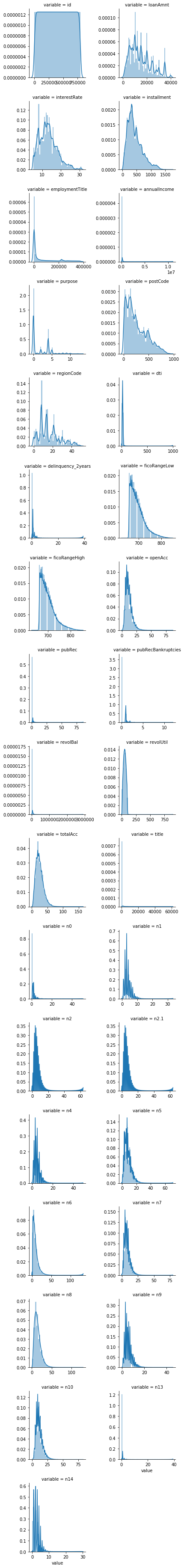
数值连续型变量分析

#每个数字特征得分布可视化
f = pd.melt(data_train, value_vars=numerical_serial_fea)
g = sns.FacetGrid(f, col="variable",  col_wrap=2, sharex=False, sharey=False)
g = g.map(sns.distplot, "value")

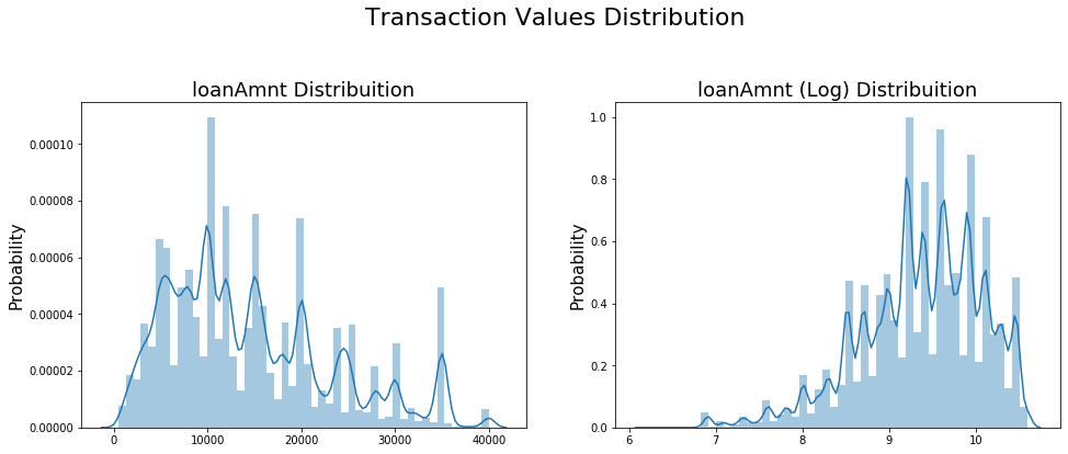
查看某一个数值型变量的分布，查看变量是否符合正态分布，如果不符合正太分布的变量可以log化后再观察下是否符合正态分布。
如果想统一处理一批数据变标准化必须把这些之前已经正态化的数据提出
正态化的原因：一些情况下正态非正态可以让模型更快的收敛，一些模型要求数据正态（eg. GMM、KNN）,保证数据不要过偏态即可，过于偏态可能会影响模型预测结果。

#Ploting Transaction Amount Values Distribution
plt.figure(figsize=(16,12))
plt.suptitle('Transaction Values Distribution', fontsize=22)
plt.subplot(221)
sub_plot_1 = sns.distplot(data_train['loanAmnt'])
sub_plot_1.set_title("loanAmnt Distribuition", fontsize=18)
sub_plot_1.set_xlabel("")
sub_plot_1.set_ylabel("Probability", fontsize=15)

plt.subplot(222)
sub_plot_2 = sns.distplot(np.log(data_train['loanAmnt']))
sub_plot_2.set_title("loanAmnt (Log) Distribuition", fontsize=18)
sub_plot_2.set_xlabel("")
sub_plot_2.set_ylabel("Probability", fontsize=15)

Text(0, 0.5, 'Probability')

非数值类别型变量分析

category_fea

['grade', 'subGrade', 'employmentLength', 'issueDate', 'earliesCreditLine']

data_train['grade'].value_counts()

B    233690
C    227118
A    139661
D    119453
E     55661
F     19053
G      5364
Name: grade, dtype: int64

data_train['subGrade'].value_counts()

C1    50763
B4    49516
B5    48965
B3    48600
C2    47068
C3    44751
C4    44272
B2    44227
B1    42382
C5    40264
A5    38045
A4    30928
D1    30538
D2    26528
A1    25909
D3    23410
A3    22655
A2    22124
D4    21139
D5    17838
E1    14064
E2    12746
E3    10925
E4     9273
E5     8653
F1     5925
F2     4340
F3     3577
F4     2859
F5     2352
G1     1759
G2     1231
G3      978
G4      751
G5      645
Name: subGrade, dtype: int64

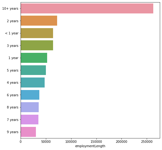
data_train['employmentLength'].value_counts()

10+ years    262753
2 years       72358
< 1 year      64237
3 years       64152
1 year        52489
5 years       50102
4 years       47985
6 years       37254
8 years       36192
7 years       35407
9 years       30272
Name: employmentLength, dtype: int64

data_train['issueDate'].value_counts()

2016-03-01    29066
2015-10-01    25525
2015-07-01    24496
2015-12-01    23245
2014-10-01    21461
              ...  
2007-08-01       23
2007-07-01       21
2008-09-01       19
2007-09-01        7
2007-06-01        1
Name: issueDate, Length: 139, dtype: int64

data_train['earliesCreditLine'].value_counts()

Aug-2001    5567
Sep-2003    5403
Aug-2002    5403
Oct-2001    5258
Aug-2000    5246
            ... 
May-1960       1
Apr-1958       1
Feb-1960       1
Aug-1946       1
Mar-1958       1
Name: earliesCreditLine, Length: 720, dtype: int64

data_train['isDefault'].value_counts()

0    640390
1    159610
Name: isDefault, dtype: int64

2.1.4 小结：

上面我们用value_counts()等函数看了特征属性的分布，但是图表是概括原始信息最便捷的方式。
数无形时少直觉。
同一份数据集，在不同的尺度刻画上显示出来的图形反映的规律是不一样的。python将数据转化成图表，但结论是否正确需要由你保证。

2.2 变量分布可视化

2.2.1单一变量分布可视化

plt.figure(figsize=(8, 8))
sns.barplot(data_train["employmentLength"].value_counts(dropna=False)[:20],
            data_train["employmentLength"].value_counts(dropna=False).keys()[:20])
plt.show()

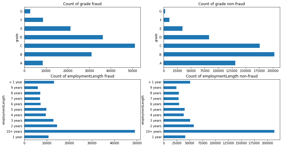
2.2.2根绝y值不同可视化x某个特征的分布

首先查看类别型变量在不同y值上的分布

train_loan_fr = data_train.loc[data_train['isDefault'] == 1]
train_loan_nofr = data_train.loc[data_train['isDefault'] == 0]

fig, ((ax1, ax2), (ax3, ax4)) = plt.subplots(2, 2, figsize=(15, 8))
train_loan_fr.groupby('grade')['grade'].count().plot(kind='barh', ax=ax1, title='Count of grade fraud')
train_loan_nofr.groupby('grade')['grade'].count().plot(kind='barh', ax=ax2, title='Count of grade non-fraud')
train_loan_fr.groupby('employmentLength')['employmentLength'].count().plot(kind='barh', ax=ax3, title='Count of employmentLength fraud')
train_loan_nofr.groupby('employmentLength')['employmentLength'].count().plot(kind='barh', ax=ax4, title='Count of employmentLength non-fraud')
plt.show()

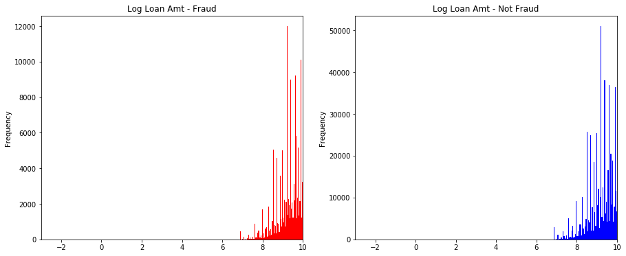
其次查看连续型变量在不同y值上的分布

fig, ((ax1, ax2)) = plt.subplots(1, 2, figsize=(15, 6))
data_train.loc[data_train['isDefault'] == 1] \
    ['loanAmnt'].apply(np.log) \
    .plot(kind='hist',
          bins=100,
          title='Log Loan Amt - Fraud',
          color='r',
          xlim=(-3, 10),
         ax= ax1)
data_train.loc[data_train['isDefault'] == 0] \
    ['loanAmnt'].apply(np.log) \
    .plot(kind='hist',
          bins=100,
          title='Log Loan Amt - Not Fraud',
          color='b',
          xlim=(-3, 10),
         ax=ax2)

<matplotlib.axes._subplots.AxesSubplot at 0x126a44b50>

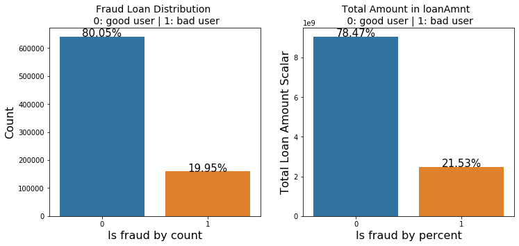
total = len(data_train)
total_amt = data_train.groupby(['isDefault'])['loanAmnt'].sum().sum()
plt.figure(figsize=(12,5))
plt.subplot(121)##1代表行，2代表列，所以一共有2个图，1代表此时绘制第一个图。
plot_tr = sns.countplot(x='isDefault',data=data_train)#data_train‘isDefault’这个特征每种类别的数量**
plot_tr.set_title("Fraud Loan Distribution \n 0: good user | 1: bad user", fontsize=14)
plot_tr.set_xlabel("Is fraud by count", fontsize=16)
plot_tr.set_ylabel('Count', fontsize=16)
for p in plot_tr.patches:
    height = p.get_height()
    plot_tr.text(p.get_x()+p.get_width()/2.,
            height + 3,
            '{:1.2f}%'.format(height/total*100),
            ha="center", fontsize=15) 
    
percent_amt = (data_train.groupby(['isDefault'])['loanAmnt'].sum())
percent_amt = percent_amt.reset_index()
plt.subplot(122)
plot_tr_2 = sns.barplot(x='isDefault', y='loanAmnt',  dodge=True, data=percent_amt)
plot_tr_2.set_title("Total Amount in loanAmnt  \n 0: good user | 1: bad user", fontsize=14)
plot_tr_2.set_xlabel("Is fraud by percent", fontsize=16)
plot_tr_2.set_ylabel('Total Loan Amount Scalar', fontsize=16)
for p in plot_tr_2.patches:
    height = p.get_height()
    plot_tr_2.text(p.get_x()+p.get_width()/2.,
            height + 3,
            '{:1.2f}%'.format(height/total_amt * 100),
            ha="center", fontsize=15)

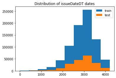
2.2.3 时间格式数据处理及查看

#转化成时间格式  issueDateDT特征表示数据日期离数据集中日期最早的日期（2007-06-01）的天数
data_train['issueDate'] = pd.to_datetime(data_train['issueDate'],format='%Y-%m-%d')
startdate = datetime.datetime.strptime('2007-06-01', '%Y-%m-%d')
data_train['issueDateDT'] = data_train['issueDate'].apply(lambda x: x-startdate).dt.days

#转化成时间格式
data_test_a['issueDate'] = pd.to_datetime(data_train['issueDate'],format='%Y-%m-%d')
startdate = datetime.datetime.strptime('2007-06-01', '%Y-%m-%d')
data_test_a['issueDateDT'] = data_test_a['issueDate'].apply(lambda x: x-startdate).dt.days

plt.hist(data_train['issueDateDT'], label='train');
plt.hist(data_test_a['issueDateDT'], label='test');
plt.legend();
plt.title('Distribution of issueDateDT dates');
#train 和 test issueDateDT 日期有重叠 所以使用基于时间的分割进行验证是不明智的

2.3.4 掌握透视图可以让我们更好的了解数据

#透视图 索引可以有多个，“columns（列）”是可选的，聚合函数aggfunc最后是被应用到了变量“values”中你所列举的项目上。
pivot = pd.pivot_table(data_train, index=['grade'], columns=['issueDateDT'], values=['loanAmnt'], aggfunc=np.sum)

pivot

2.3. 用pandas_profiling生成数据报告

import pandas_profiling

pfr = pandas_profiling.ProfileReport(data_train)
pfr.to_file("./example.html")

2.4 总结

数据探索性分析是我们初步了解数据，熟悉数据为特征工程做准备的阶段，甚至很多时候EDA阶段提取出来的特征可以直接当作规则来用。可见EDA的重要性，这个阶段的主要工作还是借助于各个简单的统计量来对数据整体的了解，分析各个类型变量相互之间的关系，以及用合适的图形可视化出来直观观察。希望本节内容能给初学者带来帮助，更期待各位学习者对其中的不足提出建议。

3.特征工程

import pandas as pd
import numpy as np
import matplotlib.pyplot as plt
import seaborn as sns
import datetime
from tqdm import tqdm
from sklearn.preprocessing import LabelEncoder
from sklearn.feature_selection import SelectKBest
from sklearn.feature_selection import chi2
from sklearn.preprocessing import MinMaxScaler
import xgboost as xgb
import lightgbm as lgb
from catboost import CatBoostRegressor
import warnings
from sklearn.model_selection import StratifiedKFold, KFold
from sklearn.metrics import accuracy_score, f1_score, roc_auc_score, log_loss
warnings.filterwarnings('ignore')

data_train =pd.read_csv('../train.csv')
data_test_a = pd.read_csv('../testA.csv')

3.1 特征预处理

数据EDA部分我们已经对数据的大概和某些特征分布有了了解，数据预处理部分一般我们要处理一些EDA阶段分析出来的问题，这里介绍了数据缺失值的填充，时间格式特征的转化处理，某些对象类别特征的处理。

首先我们查找出数据中的对象特征和数值特征

numerical_fea = list(data_train.select_dtypes(exclude=['object']).columns)
category_fea = list(filter(lambda x: x not in numerical_fea,list(data_train.columns)))
label = 'isDefault'
numerical_fea.remove(label)

在比赛中数据预处理是必不可少的一部分，对于缺失值的填充往往会影响比赛的结果，在比赛中不妨尝试多种填充然后比较结果选择结果最优的一种；
比赛数据相比真实场景的数据相对要“干净”一些，但是还是会有一定的“脏”数据存在，清洗一些异常值往往会获得意想不到的效果。

把所有缺失值替换为指定的值0

data_train = data_train.fillna(0)
向用缺失值上面的值替换缺失值

data_train = data_train.fillna(axis=0,method='ffill')
纵向用缺失值下面的值替换缺失值,且设置最多只填充两个连续的缺失值

data_train = data_train.fillna(axis=0,method='bfill',limit=2)

#查看缺失值情况
data_train.isnull().sum()

#按照平均数填充数值型特征
data_train[numerical_fea] = data_train[numerical_fea].fillna(data_train[numerical_fea].median())
data_test_a[numerical_fea] = data_test_a[numerical_fea].fillna(data_train[numerical_fea].median())
#按照众数填充类别型特征
data_train[category_fea] = data_train[category_fea].fillna(data_train[category_fea].mode())
data_test_a[category_fea] = data_test_a[category_fea].fillna(data_train[category_fea].mode())

data_train.isnull().sum()

#查看类别特征
category_fea

['grade', 'subGrade', 'employmentLength', 'issueDate', 'earliesCreditLine']

category_fea：对象型类别特征需要进行预处理，其中['issueDate']为时间格式特征。

#转化成时间格式
for data in [data_train, data_test_a]:
    data['issueDate'] = pd.to_datetime(data['issueDate'],format='%Y-%m-%d')
    startdate = datetime.datetime.strptime('2007-06-01', '%Y-%m-%d')
    #构造时间特征
    data['issueDateDT'] = data['issueDate'].apply(lambda x: x-startdate).dt.days

data_train['employmentLength'].value_counts(dropna=False).sort_index()

1 year        52489
10+ years    262753
2 years       72358
3 years       64152
4 years       47985
5 years       50102
6 years       37254
7 years       35407
8 years       36192
9 years       30272
< 1 year      64237
NaN           46799
Name: employmentLength, dtype: int64

def employmentLength_to_int(s):
    if pd.isnull(s):
        return s
    else:
        return np.int8(s.split()[0])
for data in [data_train, data_test_a]:
    data['employmentLength'].replace(to_replace='10+ years', value='10 years', inplace=True)
    data['employmentLength'].replace('< 1 year', '0 years', inplace=True)
    data['employmentLength'] = data['employmentLength'].apply(employmentLength_to_int)

data['employmentLength'].value_counts(dropna=False).sort_index()

0.0     15989
1.0     13182
2.0     18207
3.0     16011
4.0     11833
5.0     12543
6.0      9328
7.0      8823
8.0      8976
9.0      7594
10.0    65772
NaN     11742
Name: employmentLength, dtype: int64

对earliesCreditLine进行预处理

data_train['earliesCreditLine'].sample(5)

519915    Sep-2002
564368    Dec-1996
768209    May-2004
453092    Nov-1995
763866    Sep-2000
Name: earliesCreditLine, dtype: object

for data in [data_train, data_test_a]:
    data['earliesCreditLine'] = data['earliesCreditLine'].apply(lambda s: int(s[-4:]))

# 部分类别特征
cate_features = ['grade', 'subGrade', 'employmentTitle', 'homeOwnership', 'verificationStatus', 'purpose', 'postCode', 'regionCode', \
                 'applicationType', 'initialListStatus', 'title', 'policyCode']
for f in cate_features:
    print(f, '类型数：', data[f].nunique())

grade 类型数： 7
subGrade 类型数： 35
employmentTitle 类型数： 79282
homeOwnership 类型数： 6
verificationStatus 类型数： 3
purpose 类型数： 14
postCode 类型数： 889
regionCode 类型数： 51
applicationType 类型数： 2
initialListStatus 类型数： 2
title 类型数： 12058
policyCode 类型数： 1

像等级这种类别特征，是有优先级的可以labelencode或者自映射

for data in [data_train, data_test_a]:
    data['grade'] = data['grade'].map({'A':1,'B':2,'C':3,'D':4,'E':5,'F':6,'G':7})

# 类型数在2之上，又不是高维稀疏的,且纯分类特征
for data in [data_train, data_test_a]:
    data = pd.get_dummies(data, columns=['subGrade', 'homeOwnership', 'verificationStatus', 'purpose', 'regionCode'], drop_first=True)

3.2 异常值处理

当你发现异常值后，一定要先分清是什么原因导致的异常值，然后再考虑如何处理。首先，如果这一异常值并不代表一种规律性的，而是极其偶然的现象，或者说你并不想研究这种偶然的现象，这时可以将其删除。其次，如果异常值存在且代表了一种真实存在的现象，那就不能随便删除。在现有的欺诈场景中很多时候欺诈数据本身相对于正常数据勒说就是异常的，我们要把这些异常点纳入，重新拟合模型，研究其规律。能用监督的用监督模型，不能用的还可以考虑用异常检测的算法来做。
注意test的数据不能删。

3.2.1 检测异常的方法一：均方差

在统计学中，如果一个数据分布近似正态，那么大约 68% 的数据值会在均值的一个标准差范围内，大约 95% 会在两个标准差范围内，大约 99.7% 会在三个标准差范围内。

def find_outliers_by_3segama(data,fea):
    data_std = np.std(data[fea])
    data_mean = np.mean(data[fea])
    outliers_cut_off = data_std * 3
    lower_rule = data_mean - outliers_cut_off
    upper_rule = data_mean + outliers_cut_off
    data[fea+'_outliers'] = data[fea].apply(lambda x:str('异常值') if x > upper_rule or x < lower_rule else '正常值')
    return data

得到特征的异常值后可以进一步分析变量异常值和目标变量的关系

data_train = data_train.copy()
for fea in numerical_fea:
    data_train = find_outliers_by_3segama(data_train,fea)
    print(data_train[fea+'_outliers'].value_counts())
    print(data_train.groupby(fea+'_outliers')['isDefault'].sum())
    print('*'*10)

例如可以看到异常值在两个变量上的分布几乎复合整体的分布，如果异常值都属于为1的用户数据里面代表什么呢？

#删除异常值
for fea in numerical_fea:
    data_train = data_train[data_train[fea+'_outliers']=='正常值']
    data_train = data_train.reset_index(drop=True)

3.2.1检测异常的方法二：箱型图

总结一句话：四分位数会将数据分为三个点和四个区间，IQR = Q3 -Q1，下触须=Q1 ? 1.5x IQR，上触须=Q3 + 1.5x IQR；

3.3 数据分桶

特征分箱的目的：
- 从模型效果上来看，特征分箱主要是为了降低变量的复杂性，减少变量噪音对模型的影响，提高自变量和因变量的相关度。从而使模型更加稳定。
数据分桶的对象：
- 将连续变量离散化
- 将多状态的离散变量合并成少状态
分箱的原因：
- 数据的特征内的值跨度可能比较大，对有监督和无监督中如k-均值聚类它使用欧氏距离作为相似度函数来测量数据点之间的相似度。都会造成大吃小的影响，其中一种解决方法是对计数值进行区间量化即数据分桶也叫做数据分箱，然后使用量化后的结果。
分箱的优点：
- 处理缺失值：当数据源可能存在缺失值，此时可以把null单独作为一个分箱。
- 处理异常值：当数据中存在离群点时，可以把其通过分箱离散化处理，从而提高变量的鲁棒性（抗干扰能力）。例如，age若出现200这种异常值，可分入“age > 60”这个分箱里，排除影响。
- 业务解释性：我们习惯于线性判断变量的作用，当x越来越大，y就越来越大。但实际x与y之间经常存在着非线性关系，此时可经过WOE变换。
特别要注意一下分箱的基本原则：
- （1）最小分箱占比不低于5%
- （2）箱内不能全部是好客户
- （3）连续箱单调

固定宽度分箱

当数值横跨多个数量级时，最好按照 10 的幂（或任何常数的幂）来进行分组：0_9、1099、100_999、10009999，等等。固定宽度分箱非常容易计算，但如果计数值中有比较大的缺口，就会产生很多没有任何数据的空箱子。

#通过除法映射到间隔均匀的分箱中，每个分箱的取值范围都是loanAmnt/1000
data['loanAmnt_bin1'] = np.floor_divide(data['loanAmnt'], 1000)

##通过对数函数映射到指数宽度分箱
data['loanAmnt_bin2'] = np.floor(np.log10(data['loanAmnt']))

分位数分箱

data['loanAmnt_bin3'] = pd.qcut(data['loanAmnt'], 10, labels=False)

卡方分箱及其他分箱方法的尝试

这一部分属于进阶部分，学有余力的同学可以自行搜索尝试。

3.4 特征交互

交互特征的构造非常简单，使用起来却代价不菲。如果线性模型中包含有交互特征对，那它的训练时间和评分时间就会从 O(n) 增加到 O(n2)，其中 n 是单一特征的数量。

for col in ['grade', 'subGrade']: 
    temp_dict = data_train.groupby([col])['isDefault'].agg(['mean']).reset_index().rename(columns={'mean': col + '_target_mean'})
    temp_dict.index = temp_dict[col].values
    temp_dict = temp_dict[col + '_target_mean'].to_dict()

    data_train[col + '_target_mean'] = data_train[col].map(temp_dict)
    data_test_a[col + '_target_mean'] = data_test_a[col].map(temp_dict)

# 其他衍生变量 mean 和 std
for df in [data_train, data_test_a]:
    for item in ['n0','n1','n2','n2.1','n4','n5','n6','n7','n8','n9','n10','n11','n12','n13','n14']:
        df['grade_to_mean_' + item] = df['grade'] / df.groupby([item])['grade'].transform('mean')
        df['grade_to_std_' + item] = df['grade'] / df.groupby([item])['grade'].transform('std')

这里给出一些特征交互的思路，但特征和特征间的交互衍生出新的特征还远远不止于此，抛砖引玉，希望大家多多探索。请学习者尝试其他的特征交互方法。

3.5 特征编码

3.5.1labelEncode 直接放入树模型中

#label-encode:subGrade,postCode,title
#高维类别特征需要进行转换
for col in tqdm(['employmentTitle', 'postCode', 'title','subGrade']):
    le = LabelEncoder()
    le.fit(list(data_train[col].astype(str).values) + list(data_test_a[col].astype(str).values))
    data_train[col] = le.transform(list(data_train[col].astype(str).values))
    data_test_a[col] = le.transform(list(data_test_a[col].astype(str).values))
print('Label Encoding 完成')

100%|██████████| 4/4 [00:08<00:00,  2.04s/it]

Label Encoding 完成

3.5.2逻辑回归等模型要单独增加的特征工程

对特征做归一化，去除相关性高的特征
归一化目的是让训练过程更好更快的收敛，避免特征大吃小的问题
去除相关性是增加模型的可解释性，加快预测过程。

# 举例归一化过程
#伪代码
for fea in [要归一化的特征列表]：
    data[fea] = ((data[fea] - np.min(data[fea])) / (np.max(data[fea]) - np.min(data[fea])))

3.6 特征选择

特征选择技术可以精简掉无用的特征，以降低最终模型的复杂性，它的最终目的是得到一个简约模型，在不降低预测准确率或对预测准确率影响不大的情况下提高计算速度。特征选择不是为了减少训练时间（实际上，一些技术会增加总体训练时间），而是为了减少模型评分时间。

特征选择的方法：

1 Filter
- 方差选择法
- 相关系数法（pearson 相关系数）
- 卡方检验
- 互信息法
2 Wrapper （RFE）
- 递归特征消除法
3 Embedded
- 基于惩罚项的特征选择法
- 基于树模型的特征选择

3.6.1Filter（方差选择法、相关系数法）

基于特征间的关系进行筛选

方差选择法

方差选择法中，先要计算各个特征的方差，然后根据设定的阈值，选择方差大于阈值的特征

from sklearn.feature_selection import VarianceThreshold
#其中参数threshold为方差的阈值
VarianceThreshold(threshold=3).fit_transform(train,target_train)

3.6.2Wrapper （递归特征法）

递归特征消除法递归消除特征法使用一个基模型来进行多轮训练，每轮训练后，消除若干权值系数的特征，再基于新的特征集进行下一轮训练。在feature_selection库的RFE类可以用于选择特征，相关代码如下（以逻辑回归为例）：

from sklearn.feature_selection import RFE
from sklearn.linear_model import LogisticRegression
#递归特征消除法，返回特征选择后的数据
#参数estimator为基模型
#参数n_features_to_select为选择的特征个数

RFE(estimator=LogisticRegression(), n_features_to_select=2).fit_transform(train,target_train)

3.6.3Embedded（惩罚项的特征选择法、树模型的特征选择）

基于惩罚项的特征选择法使用带惩罚项的基模型，除了筛选出特征外，同时也进行了降维。在feature_selection库的SelectFromModel类结合逻辑回归模型可以用于选择特征，相关代码如下：

from sklearn.feature_selection import SelectFromModel
from sklearn.linear_model import LogisticRegression
#带L1惩罚项的逻辑回归作为基模型的特征选择

SelectFromModel(LogisticRegression(penalty="l1", C=0.1)).fit_transform(train,target_train)

基于树模型的特征选择树模型中GBDT也可用来作为基模型进行特征选择。在feature_selection库的SelectFromModel类结合GBDT模型可以用于选择特征，相关代码如下：

from sklearn.feature_selection import SelectFromModel
from sklearn.ensemble import GradientBoostingClassifier
#GBDT作为基模型的特征选择
SelectFromModel(GradientBoostingClassifier()).fit_transform(train,target_train)

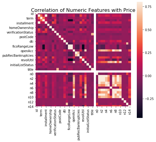
本数据集中我们删除非入模特征后，并对缺失值填充，然后用计算协方差的方式看一下特征间相关性，然后进行模型训练

# 删除不需要的数据
for data in [data_train, data_test_a]:
    data.drop(['issueDate','id'], axis=1,inplace=True)

"纵向用缺失值上面的值替换缺失值"
data_train = data_train.fillna(axis=0,method='ffill')

x_train = data_train.drop(['isDefault','id'], axis=1)
#计算协方差
data_corr = x_train.corrwith(data_train.isDefault) #计算相关性
result = pd.DataFrame(columns=['features', 'corr'])
result['features'] = data_corr.index
result['corr'] = data_corr.values

# 当然也可以直接看图
data_numeric = data_train[numerical_fea]
correlation = data_numeric.corr()

f , ax = plt.subplots(figsize = (7, 7))
plt.title('Correlation of Numeric Features with Price',y=1,size=16)
sns.heatmap(correlation,square = True,  vmax=0.8)

<matplotlib.axes._subplots.AxesSubplot at 0x12d88ad10>

features = [f for f in data_train.columns if f not in ['id','issueDate','isDefault'] and '_outliers' not in f]
x_train = data_train[features]
x_test = data_test_a[features]
y_train = data_train['isDefault']

def cv_model(clf, train_x, train_y, test_x, clf_name):
    folds = 5
    seed = 2020
    kf = KFold(n_splits=folds, shuffle=True, random_state=seed)

    train = np.zeros(train_x.shape[0])
    test = np.zeros(test_x.shape[0])

    cv_scores = []

    for i, (train_index, valid_index) in enumerate(kf.split(train_x, train_y)):
        print('************************************ {} ************************************'.format(str(i+1)))
        trn_x, trn_y, val_x, val_y = train_x.iloc[train_index], train_y[train_index], train_x.iloc[valid_index], train_y[valid_index]

        if clf_name == "lgb":
            train_matrix = clf.Dataset(trn_x, label=trn_y)
            valid_matrix = clf.Dataset(val_x, label=val_y)

            params = {
                'boosting_type': 'gbdt',
                'objective': 'binary',
                'metric': 'auc',
                'min_child_weight': 5,
                'num_leaves': 2 ** 5,
                'lambda_l2': 10,
                'feature_fraction': 0.8,
                'bagging_fraction': 0.8,
                'bagging_freq': 4,
                'learning_rate': 0.1,
                'seed': 2020,
                'nthread': 28,
                'n_jobs':24,
                'silent': True,
                'verbose': -1,
            }

            model = clf.train(params, train_matrix, 50000, valid_sets=[train_matrix, valid_matrix], verbose_eval=200,early_stopping_rounds=200)
            val_pred = model.predict(val_x, num_iteration=model.best_iteration)
            test_pred = model.predict(test_x, num_iteration=model.best_iteration)
            
            # print(list(sorted(zip(features, model.feature_importance("gain")), key=lambda x: x[1], reverse=True))[:20])
                
        if clf_name == "xgb":
            train_matrix = clf.DMatrix(trn_x , label=trn_y)
            valid_matrix = clf.DMatrix(val_x , label=val_y)
            
            params = {'booster': 'gbtree',
                      'objective': 'binary:logistic',
                      'eval_metric': 'auc',
                      'gamma': 1,
                      'min_child_weight': 1.5,
                      'max_depth': 5,
                      'lambda': 10,
                      'subsample': 0.7,
                      'colsample_bytree': 0.7,
                      'colsample_bylevel': 0.7,
                      'eta': 0.04,
                      'tree_method': 'exact',
                      'seed': 2020,
                      'nthread': 36,
                      "silent": True,
                      }
            
            watchlist = [(train_matrix, 'train'),(valid_matrix, 'eval')]
            
            model = clf.train(params, train_matrix, num_boost_round=50000, evals=watchlist, verbose_eval=200, early_stopping_rounds=200)
            val_pred  = model.predict(valid_matrix, ntree_limit=model.best_ntree_limit)
            test_pred = model.predict(test_x , ntree_limit=model.best_ntree_limit)
                 
        if clf_name == "cat":
            params = {'learning_rate': 0.05, 'depth': 5, 'l2_leaf_reg': 10, 'bootstrap_type': 'Bernoulli',
                      'od_type': 'Iter', 'od_wait': 50, 'random_seed': 11, 'allow_writing_files': False}
            
            model = clf(iterations=20000, **params)
            model.fit(trn_x, trn_y, eval_set=(val_x, val_y),
                      cat_features=[], use_best_model=True, verbose=500)
            
            val_pred  = model.predict(val_x)
            test_pred = model.predict(test_x)
            
        train[valid_index] = val_pred
        test = test_pred / kf.n_splits
        cv_scores.append(roc_auc_score(val_y, val_pred))
        
        print(cv_scores)
        
    print("%s_scotrainre_list:" % clf_name, cv_scores)
    print("%s_score_mean:" % clf_name, np.mean(cv_scores))
    print("%s_score_std:" % clf_name, np.std(cv_scores))
    return train, test

def lgb_model(x_train, y_train, x_test):
    lgb_train, lgb_test = cv_model(lgb, x_train, y_train, x_test, "lgb")
    return lgb_train, lgb_test

def xgb_model(x_train, y_train, x_test):
    xgb_train, xgb_test = cv_model(xgb, x_train, y_train, x_test, "xgb")
    return xgb_train, xgb_test

def cat_model(x_train, y_train, x_test):
    cat_train, cat_test = cv_model(CatBoostRegressor, x_train, y_train, x_test, "cat")

lgb_train, lgb_test = lgb_model(x_train, y_train, x_test)

************************************ 1 ************************************
Training until validation scores don't improve for 200 rounds
[200]	training's auc: 0.749225	valid_1's auc: 0.729679
[400]	training's auc: 0.765075	valid_1's auc: 0.730496
[600]	training's auc: 0.778745	valid_1's auc: 0.730435
Early stopping, best iteration is:
[455]	training's auc: 0.769202	valid_1's auc: 0.730686
[0.7306859913754798]
************************************ 2 ************************************
Training until validation scores don't improve for 200 rounds
[200]	training's auc: 0.749221	valid_1's auc: 0.731315
[400]	training's auc: 0.765117	valid_1's auc: 0.731658
[600]	training's auc: 0.778542	valid_1's auc: 0.731333
Early stopping, best iteration is:
[407]	training's auc: 0.765671	valid_1's auc: 0.73173
[0.7306859913754798, 0.7317304414673989]
************************************ 3 ************************************
Training until validation scores don't improve for 200 rounds
[200]	training's auc: 0.748436	valid_1's auc: 0.732775
[400]	training's auc: 0.764216	valid_1's auc: 0.733173
Early stopping, best iteration is:
[386]	training's auc: 0.763261	valid_1's auc: 0.733261
[0.7306859913754798, 0.7317304414673989, 0.7332610441015461]
************************************ 4 ************************************
Training until validation scores don't improve for 200 rounds
[200]	training's auc: 0.749631	valid_1's auc: 0.728327
[400]	training's auc: 0.765139	valid_1's auc: 0.728845
Early stopping, best iteration is:
[286]	training's auc: 0.756978	valid_1's auc: 0.728976
[0.7306859913754798, 0.7317304414673989, 0.7332610441015461, 0.7289759386807912]
************************************ 5 ************************************
Training until validation scores don't improve for 200 rounds
[200]	training's auc: 0.748414	valid_1's auc: 0.732727
[400]	training's auc: 0.763727	valid_1's auc: 0.733531
[600]	training's auc: 0.777489	valid_1's auc: 0.733566
Early stopping, best iteration is:
[524]	training's auc: 0.772372	valid_1's auc: 0.733772
[0.7306859913754798, 0.7317304414673989, 0.7332610441015461, 0.7289759386807912, 0.7337723979789789]
lgb_scotrainre_list: [0.7306859913754798, 0.7317304414673989, 0.7332610441015461, 0.7289759386807912, 0.7337723979789789]
lgb_score_mean: 0.7316851627208389
lgb_score_std: 0.0017424259863954693

testA_result = pd.read_csv('../testA_result.csv')

roc_auc_score(testA_result['isDefault'].values, lgb_test)

0.7290917729487896

3.8总结

特征工程是机器学习，甚至是深度学习中最为重要的一部分，在实际应用中往往也是所花费时间最多的一步。各种算法书中对特征工程部分的讲解往往少得可怜，因为特征工程和具体的数据结合的太紧密，很难系统地覆盖所有场景。本章主要是通过一些常用的方法来做介绍，例如缺失值异常值的处理方法详细对任何数据集来说都是适用的。但对于分箱等操作本章给出了具体的几种思路，需要读者自己探索。在特征工程中比赛和具体的应用还是有所不同的，在实际的金融风控评分卡制作过程中，由于强调特征的可解释性，特征分箱尤其重要。

项目链接以及码源

数据挖掘专栏

数据挖掘实践（金融风控）：金融风控之贷款违约预测挑战赛(上篇)

数据挖掘实践（金融风控）：金融风控之贷款违约预测挑战赛(下篇)

posted @ 2023-05-17 15:27 汀、人工智能阅读(1) 评论(0) 编辑收藏举报

数据挖掘实践（金融风控）：金融风控之贷款违约预测挑战赛（上篇）[xgboots/lightgbm/Catboost等模型]--模型融合：stacking、blending

数据挖掘实践（金融风控）：金融风控之贷款违约预测挑战赛（上篇）[xgboots/lightgbm/Catboost等模型]--模型融合：stacking、blending

数据挖掘实践（金融风控）：金融风控之贷款违约预测挑战赛（上篇）[xgboots/lightgbm/Catboost等模型]--模型融合：stacking、blending

1.赛题简介

项目链接以及码源见文末

1.1数据介绍

1.2预测指标

1.2.1 分类算法常见的评估指标如下：

1.2.2 对于金融风控预测类常见的评估指标如下:

1.3 项目流程介绍

1.4 代码示例

1.4.1 数据读取pandas

1.4.2 分类指标评价计算示例

1.5 拓展知识——评分卡

2.数据探索性分析

2.1 代码示例

2.1.1 导入数据分析及可视化过程需要的库

2.1.2 读取文件

查看数据集的样本个数和原始特征维度

2.1.3查看数据集中特征缺失值，唯一值等

2.1.4 查看特征的数值类型有哪些，对象类型有哪些

2.1.4 小结：

2.2 变量分布可视化

2.2.1单一变量分布可视化

2.2.2根绝y值不同可视化x某个特征的分布

2.2.3 时间格式数据处理及查看

2.3.4 掌握透视图可以让我们更好的了解数据

2.3. 用pandas_profiling生成数据报告

2.4 总结

3.特征工程

3.1 特征预处理

3.2 异常值处理

3.2.1 检测异常的方法一：均方差

3.2.1检测异常的方法二：箱型图

3.3 数据分桶

3.4 特征交互

3.5 特征编码

3.5.1labelEncode 直接放入树模型中

3.5.2逻辑回归等模型要单独增加的特征工程

3.6 特征选择

3.6.1Filter（方差选择法、相关系数法）

3.6.2Wrapper （递归特征法）

3.6.3Embedded（ 惩罚项的特征选择法、树模型的特征选择）

3.8总结

项目链接以及码源

优雅殿下 （王者 段位）

温馨提示

最新会员

3.6.3Embedded（惩罚项的特征选择法、树模型的特征选择）

优雅殿下（王者段位）