A First course in FEM —— matlab代码实现求解传热问题(稳态)
这篇文章会将FEM全流程走一遍,包括网格、矩阵组装、求解、后处理。内容是大三时的大作业,今天拿出来回顾下。
1. 问题简介
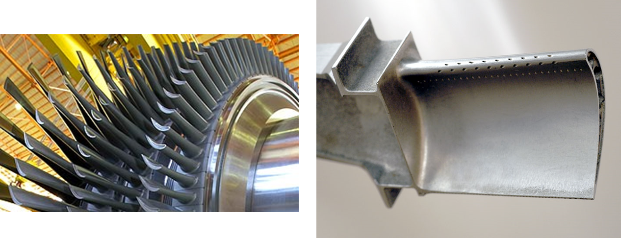
涡轮机叶片需要冷却以提高涡轮的性能和涡轮叶片的寿命。我们现在考虑一个如上图所示的叶片,叶片处在一个高温环境中,中间通有四个冷却孔。
假设为稳态,那么叶片内导热微分方程为:
内部区域: ![]() (扩散方程)
(扩散方程)
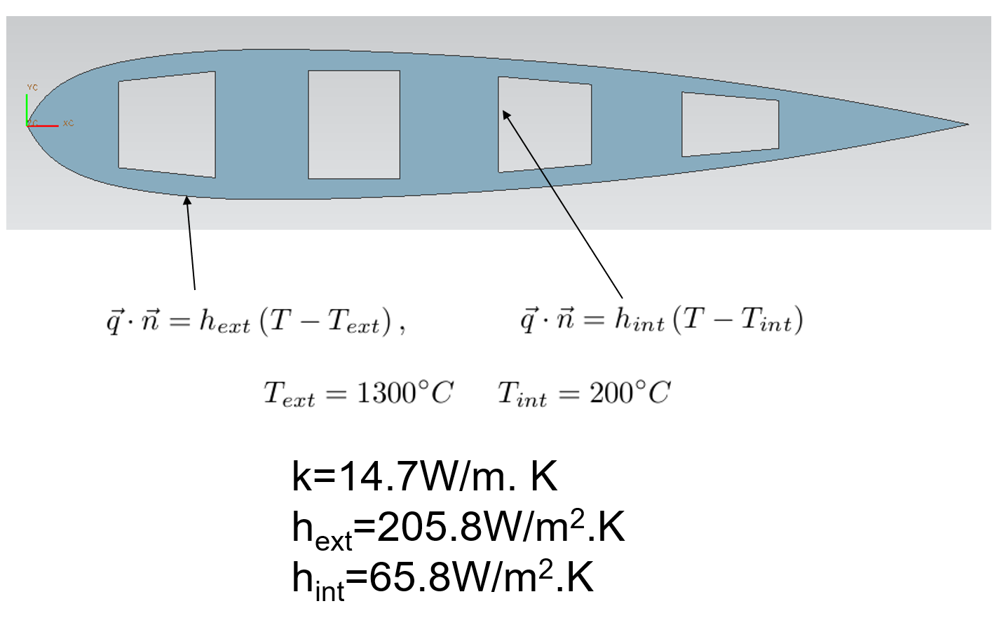
边界:
![]() (外表面)
(外表面)
![]() (内部冷却孔)
(内部冷却孔)
2.模型
2.1几何模型
我们简化为二维模型,如下图所示:
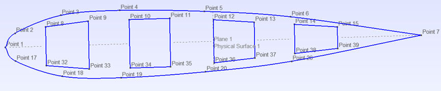
点坐标:
1:0.0,0.0 6:597.6,45.9 11:344.7,50.0
2:20.9,28.8 7:870.0,0.0 12:435.8,44.5
3:117.4,62.9 8:85.0,40.0 13:521.2,37.0
4:240.4,69.6 9:174.5,49.4 14:605.0,30.0
5:417.5,62.4 10:260.0,50.0 15:694.7,22.2
2.2 单位系统和物性
长度单位:mm
温度单位: K
功率单位:W
k=14.7*10^-3 W/mm. K
hext=205.8*10^-6 W/m2.K
hint=65.8*10^-6 W/m2.K
注意:在后面的矩阵组装中的h_wall = h / k
2.3网格
用开源软件Gmsh生成网格。
首先写geo文件
注意要把外表面和中间空洞用Physical Line定义
lc = 10;
Point(1) = {0, 0, 0, lc};
Point(2) = {20.9,28.8,0, lc};
Point(3) = {117.4,62.9,0, lc};
Point(4) = {240.4,69.6,0, lc};
Point(5) =  {417.5,62.4,0, lc};
Point(6) = {597.6,45.9,0, lc};
Point(7) = {870.0,0.0, 0,lc};
Point(8) = {85.0,40.0, 0,lc};
Point(9) = {174.5,49.4,0, lc};
Point(10) = {260.0,50.0,0, lc};
Point(11) = {344.7,50.0,0, lc};
Point(12) = {435.8,44.5,0, lc};
Point(13) = {521.2,37.0,0, lc};
Point(14) = {605.0,30.0,0, lc};
Point(15) = {694.7,22.2,0, lc};

//+
Spline(1) = {1, 2, 3, 4, 5, 6, 7};
//+
Symmetry {0, 1, 0, 0} {
  Duplicata { Point{1}; Point{2}; Point{3}; Point{4}; Point{5}; Line{1}; Point{6}; Point{7}; Point{8}; Point{9}; Point{10}; Point{11}; Point{12}; Point{13}; Point{14}; Point{15}; }
}

//+
Line Loop(1) = {1, -2};
//+
Line(3) = {8, 9};
//+
Line(4) = {9, 33};
//+
Line(5) = {33, 32};
//+
Line(6) = {32, 8};
//+
Line(7) = {10, 11};
//+
Line(8) = {11, 35};
//+
Line(9) = {35, 34};
//+
Line(10) = {34, 10};
//+
Line(11) = {12, 13};
//+
Line(12) = {13, 37};
//+
Line(13) = {37, 36};
//+
Line(14) = {36, 12};
//+
Line(15) = {14, 15};
//+
Line(16) = {15, 39};
//+
Line(17) = {39, 38};
//+
Line(18) = {38, 14};
//+
Line Loop(2) = {3, 4, 5, 6};
//+
Line Loop(3) = {7, 8, 9, 10};
//+
Line Loop(4) = {11, 12, 13, 14};
//+
Line Loop(5) = {15, 16, 17, 18};
//+
Physical Line(0)={1, -2};
Physical Line(1)={3, 4, 5, 6};
Physical Line(2)={7, 8, 9, 10};
Physical Line(3)={11, 12, 13, 14};
Physical Line(4)={15, 16, 17, 18};

Plane Surface(1) = {1, 2, 3, 4, 5};
Physical Surface(1) = {1};
边界信息如何保存?
边界edges需要用标记,
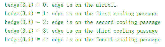
在matlab程序中用bedge(3,Nbc)存储边界信息,前两个数字代表边的两端节点编号,第三个数字代表属于哪一个边。

生成网格后导出为“blademesh.m”用以后续使用,注意不要勾选Save all elements,否则会没有边界信息。
我用gmsh-4.4.1-Windows64版本,可以导出边界信息。但是新版的gmsh导出为.m文件时,边界信息无法保存。

3. 矩阵组装
3.1 控制方程
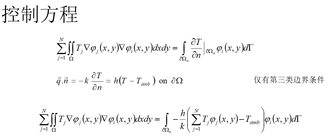
3.2 系统矩阵

其中的Ω代表全域,我们将全域分解为一个个单元,这就是有限元的思想。
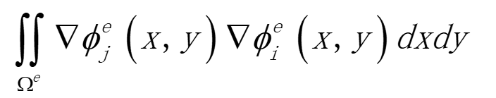
计算每个单元(Ωe)的刚度矩阵,然后每项加到整体刚度矩阵:
4. 代码实现(matlab)
|
步骤 |
工具或函数 |
|
定义求解域并生成网格 |
gmsh导出网格为blademesh.m |
|
读入网格信息,数据转换 |
bladeread |
|
矩阵和矢量组装,线性方程组求解 |
bleadheat |
|
查看结果 |
bladeplot |
主程序:bladeheat.m
% Clear variables

clear all;


% Set gas temperature and wall heat transfer coefficients at
% boundaries of the blade.  Note: Tcool(i) and hwall(i) are the
% values of Tcool and hwall for the ith boundary which are numbered
% as follows:
%
%   1 = external boundary (airfoil surface)
%   2 = 1st internal cooling passage (from leading edge)
%   3 = 2nd internal cooling passage (from leading edge)
%   3 = 3rd internal cooling passage (from leading edge)
%   3 = 4th internal cooling passage (from leading edge)

% Tcool = [1300, 200, 200, 200, 200];
% hwall = [14, 4.7, 4.7, 4.7, 4.7];

Tcool = [1573, 473, 473, 473, 473];
h = [205.8*10^-6, 65.8*10^-6, 65.8*10^-6, 65.8*10^-6, 65.8*10^-6];
k = 14.7*10^-3;
hwall = h / k;


% Load in the grid file
% NOTE:  after loading a gridfile using the load(fname) command,
%        three important grid variables and data arrays exist.  These are:
%
% Nt: Number of triangles (i.e. elements) in mesh
%
% Nv: Number of nodes (i.e. vertices) in mesh
%
% Nbc: Number of edges which lie on a boundary of the computational
%      domain.
%
% tri2nod(3,Nt):  list of the 3 node numbers which form the current
%                 triangle.  Thus, tri2nod(1,i) is the 1st node of
%                 the i'th triangle, tri2nod(2,i) is the 2nd node
%                 of the i'th triangle, etc.
%
% xy(2,Nv): list of the x and y locations of each node.  Thus,
%           xy(1,i) is the x-location of the i'th node, xy(2,i)
%           is the y-location of the i'th node, etc.
%
% bedge(3,Nbc): For each boundary edge, bedge(1,i) and bedge(2,i)
%               are the node numbers for the nodes at the end
%               points of the i'th boundary edge.  bedge(3,i) is an
%               integer which identifies which boundary the edge is
%               on. In this solver, the third value has the
%               following meaning:
%
%               bedge(3,i) = 0: edge is on the airfoil
%               bedge(3,i) = 1: edge is on the first cooling passage
%               bedge(3,i) = 2: edge is on the second cooling passage
%               bedge(3,i) = 3: edge is on the third cooling passage
%               bedge(3,i) = 4: edge is on the fourth cooling passage
%
bladeread;

% Start timer
Time0 = cputime;

% Zero stiffness matrix

K = zeros(Nv, Nv);
b = zeros(Nv, 1);

% Zero maximum element size
hmax = 0;

% Loop over elements and calculate residual and stiffness matrix

for ii = 1:Nt,

  kn(1) = tri2nod(1,ii);
  kn(2) = tri2nod(2,ii);
  kn(3) = tri2nod(3,ii);

  xe(1) = xy(1,kn(1));
  xe(2) = xy(1,kn(2));
  xe(3) = xy(1,kn(3));

  ye(1) = xy(2,kn(1));
  ye(2) = xy(2,kn(2));
  ye(3) = xy(2,kn(3));

  % Calculate circumcircle radius for the element
  % First, find the center of the circle by intersecting the median
  % segments from two of the triangle edges.

  dx21 = xe(2) - xe(1);
  dy21 = ye(2) - ye(1);

  dx31 = xe(3) - xe(1);
  dy31 = ye(3) - ye(1);

  x21  = 0.5*(xe(2) + xe(1));
  y21  = 0.5*(ye(2) + ye(1));

  x31  = 0.5*(xe(3) + xe(1));
  y31  = 0.5*(ye(3) + ye(1));

  b21 = x21*dx21 + y21*dy21;
  b31 = x31*dx31 + y31*dy31;

  xydet = dx21*dy31 - dy21*dx31;

  x0 = (dy31*b21 - dy21*b31)/xydet;
  y0 = (dx21*b31 - dx31*b21)/xydet;

  Rlocal = sqrt((xe(1)-x0)^2 + (ye(1)-y0)^2);

  if (hmax < Rlocal),
    hmax = Rlocal;
  end

  % Calculate all of the necessary shape function derivatives, the
  % Jacobian of the element, etc.

  % Derivatives of node 1's interpolant
  dNdxi(1,1) = -1.0; % with respect to xi1
  dNdxi(1,2) = -1.0; % with respect to xi2

  % Derivatives of node 2's interpolant
  dNdxi(2,1) =  1.0; % with respect to xi1
  dNdxi(2,2) =  0.0; % with respect to xi2

  % Derivatives of node 3's interpolant
  dNdxi(3,1) =  0.0; % with respect to xi1
  dNdxi(3,2) =  1.0; % with respect to xi2

  % Sum these to find dxdxi (note: these are constant within an element)
  dxdxi = zeros(2,2);
  for nn = 1:3,
    dxdxi(1,:) = dxdxi(1,:) + xe(nn)*dNdxi(nn,:);
    dxdxi(2,:) = dxdxi(2,:) + ye(nn)*dNdxi(nn,:);
  end

  % Calculate determinant for area weighting
  J = dxdxi(1,1)*dxdxi(2,2) - dxdxi(1,2)*dxdxi(2,1);
  A = 0.5*abs(J); % Area is half of the Jacobian

  % Invert dxdxi to find dxidx using inversion rule for a 2x2 matrix
  dxidx = [ dxdxi(2,2)/J, -dxdxi(1,2)/J; ...
       -dxdxi(2,1)/J,  dxdxi(1,1)/J];

  % Calculate dNdx
  dNdx = dNdxi*dxidx;

  % Add contributions to stiffness matrix for node 1 weighted residual
  K(kn(1), kn(1)) = K(kn(1), kn(1)) + (dNdx(1,1)*dNdx(1,1) + dNdx(1,2)*dNdx(1,2))*A;
  K(kn(1), kn(2)) = K(kn(1), kn(2)) + (dNdx(1,1)*dNdx(2,1) + dNdx(1,2)*dNdx(2,2))*A;
  K(kn(1), kn(3)) = K(kn(1), kn(3)) + (dNdx(1,1)*dNdx(3,1) + dNdx(1,2)*dNdx(3,2))*A;

  % Add contributions to stiffness matrix for node 2 weighted residual
  K(kn(2), kn(1)) = K(kn(2), kn(1)) + (dNdx(2,1)*dNdx(1,1) + dNdx(2,2)*dNdx(1,2))*A;
  K(kn(2), kn(2)) = K(kn(2), kn(2)) + (dNdx(2,1)*dNdx(2,1) + dNdx(2,2)*dNdx(2,2))*A;
  K(kn(2), kn(3)) = K(kn(2), kn(3)) + (dNdx(2,1)*dNdx(3,1) + dNdx(2,2)*dNdx(3,2))*A;

  % Add contributions to stiffness matrix for node 3 weighted residual
  K(kn(3), kn(1)) = K(kn(3), kn(1)) + (dNdx(3,1)*dNdx(1,1) + dNdx(3,2)*dNdx(1,2))*A;
  K(kn(3), kn(2)) = K(kn(3), kn(2)) + (dNdx(3,1)*dNdx(2,1) + dNdx(3,2)*dNdx(2,2))*A;
  K(kn(3), kn(3)) = K(kn(3), kn(3)) + (dNdx(3,1)*dNdx(3,1) + dNdx(3,2)*dNdx(3,2))*A;

end


% Loop over boundary edges and account for bc's
% Note: the bc's are all convective heat transfer coefficient bc's
% so the are of 'Robin' form.  This requires modification of the
% stiffness matrix as well as impacting the right-hand side, b.
%

for ii = 1:Nbc,

  % Get node numbers on edge
  kn(1) = bedge(1,ii);
  kn(2) = bedge(2,ii);

  % Get node coordinates
  xe(1) = xy(1,kn(1));
  xe(2) = xy(1,kn(2));

  ye(1) = xy(2,kn(1));
  ye(2) = xy(2,kn(2));

  % Calculate edge length
  ds = sqrt((xe(1)-xe(2))^2 + (ye(1)-ye(2))^2);

  % Determine the boundary number
  bnum = bedge(3,ii) + 1;

  % Based on boundary number, set heat transfer bc
  K(kn(1), kn(1)) = K(kn(1), kn(1)) + hwall(bnum)*ds*(1/3);
  K(kn(1), kn(2)) = K(kn(1), kn(2)) + hwall(bnum)*ds*(1/6);
  b(kn(1))        = b(kn(1))        + hwall(bnum)*ds*0.5*Tcool(bnum);

  K(kn(2), kn(1)) = K(kn(2), kn(1)) + hwall(bnum)*ds*(1/6);
  K(kn(2), kn(2)) = K(kn(2), kn(2)) + hwall(bnum)*ds*(1/3);
  b(kn(2))        = b(kn(2))        + hwall(bnum)*ds*0.5*Tcool(bnum);

end

% Solve for temperature
Tsol = K\b;

% Finish timer
Time1 = cputime;

% Plot solution
bladeplot;

% Report outputs
Tmax = max(Tsol);
Tmin = min(Tsol);

fprintf('Number of nodes      = %i\n',Nv);
fprintf('Number of elements   = %i\n',Nt);
fprintf('Maximum element size = %5.3f\n',hmax);
fprintf('Minimum temperature  = %6.1f\n',Tmin);
fprintf('Maximum temperature  = %6.1f\n',Tmax);
fprintf('CPU Time (secs)      = %f\n',Time1 - Time0);
bladeread.m
% Read three important grid variables and data arrays
% Nt: Number of triangles (i.e. elements) in mesh
% Nv: Number of nodes (i.e. vertices) in mesh
% Nbc: Number of edges which lie on a boundary of the computational
%      domain.
% tri2nod(3,Nt):  list of the 3 node numbers which form the current
%                 triangle.  Thus, tri2nod(1,i) is the 1st node of
%                 the i'th triangle, tri2nod(2,i) is the 2nd node
%                 of the i'th triangle, etc.
% xy(2,Nv): list of the x and y locations of each node.  Thus,
%           xy(1,i) is the x-location of the i'th node, xy(2,i)
%           is the y-location of the i'th node, etc.
% bedge(3,Nbc): For each boundary edge, bedge(1,i) and bedge(2,i)
%               are the node numbers for the nodes at the end
%               points of the i'th boundary edge.  bedge(3,i) is an
%               integer which identifies which boundary the edge is
%               on. In this solver, the third value has the
%               following meaning:
%
%               bedge(3,i) = 0: edge is on the airfoil
%               bedge(3,i) = 1: edge is on the first cooling passage
%               bedge(3,i) = 2: edge is on the second cooling passage
%               bedge(3,i) = 3: edge is on the third cooling passage
%               bedge(3,i) = 4: edge is on the fourth cooling passage
%

clc
run('blademesh.m');
Nv=msh.nbNod;
Nt=size(msh.TRIANGLES,1);
Nbc=size(msh.LINES,1);
for i=1:Nt
    tri2nod(1,i)=msh.TRIANGLES(i,1);
    tri2nod(2,i)=msh.TRIANGLES(i,2);
    tri2nod(3,i)=msh.TRIANGLES(i,3);
end
for i=1:Nv
    xy(1,i)=msh.POS(i,1);
    xy(2,i)=msh.POS(i,2);
end
for i=1:Nbc
    bedge(1,i)=msh.LINES(i,1);
    bedge(2,i)=msh.LINES(i,2);
    bedge(3,i)=msh.LINES(i,3);
end
bladeplot.m
% Plot T in triangles
figure;
for ii = 1:Nt,
  for nn = 1:3,
    xtri(nn,ii) = xy(1,tri2nod(nn,ii));
    ytri(nn,ii) = xy(2,tri2nod(nn,ii));
    Ttri(nn,ii) = Tsol(tri2nod(nn,ii));
  end
end
HT = patch(xtri,ytri,Ttri);
axis('equal');
set(HT,'LineStyle','none');
title('Temperature (K)');
% caxis([298,1573]);
colormap(jet);
HC = colorbar;
hold on; bladeplotgrid; hold off;
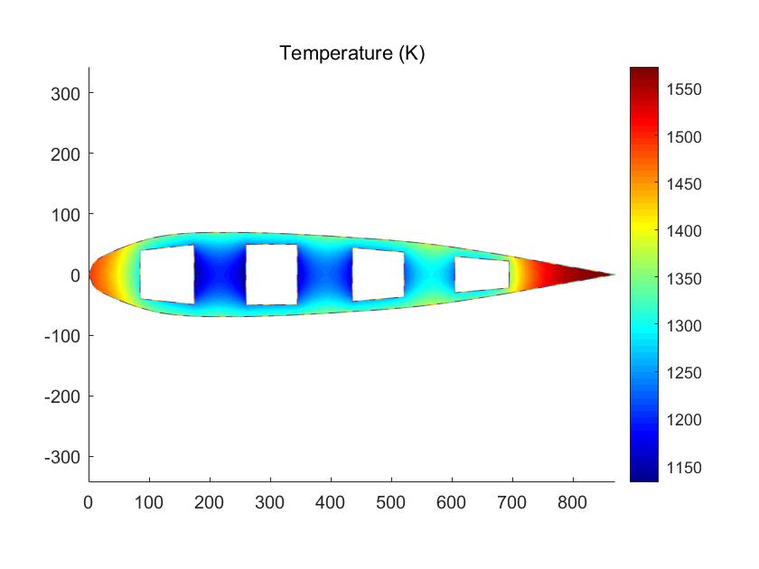
5. 计算结果