深度学习（四）之电影评论分类

任务目标

对中文电影评论进行情感分类，实现测试准确率在\(83\%\)以上。本文采用了3种模型对电影评论进行分类，最终，模型在测试集的结果分别为：

模型	acc	precision	recall	f1-score
LSTM	\(81.57\%\)	[\(77.49\%\),\(86.69\%\)]	[\(88.46\%\),\(74.87%\)]	[\(82.56\%\),\(80.46\%\)]
TextCNN	\(84.28\%\)	[\(81.96\%\),\(86.86\%\)]	[\(87.36\%\),\(81.28\%\)]	[\(84.57\%\),\(83.98\%\)]
Attention-Based BiLSTM	\(85.64\%\)	[\(85.64\%\),\(85.64\%\)]	[\(85.16\%\),\(86.10\%\)]	[\(85.40\%\),\(85.87\%\)]

实验环境：

• python：3.9.7
• pytorch：1.11.0
• numpy：1.21.2
• opencc：1.1.3 用于简繁体转换
• sklearn：1.0.2

代码地址：https://github.com/xiaohuiduan/deeplearning-study/tree/main/电影评论分类

数据集预处理

数据集一共由3个文件构成：train.txt，validation.txt和test.txt。分别用于训练，验证和测试。

部分数据如下所示，每一行代表一个样本数据，0代表好评，1代表差评。其中，每条评论都进行了预先分词处理（词与词之间使用空格进行分隔）。因此，在写代码进行数据预处理阶段并不需要对数据集的数据进行分词处理。

简繁文本转换

在电影评论数据中，存在一些繁体字，一般来说，繁体字和简体的字的意思应该是一样的。所以我们可以将繁体字转成简体字，这样在一定程度上可以减少模型的复杂度。

from opencc import OpenCCdef t2s(file_path,output_file_path):    """        file_path：源文件地址        output_file_path：转换成简体后保存的地址    """    input = open(file_path).read()    output = open(output_file_path,"w")    output.write(OpenCC("t2s").convert(input))    output.close()t2s("./data/train.txt","./data/train_zh.txt")t2s("./data/test.txt","./data/test_zh.txt")t2s("./data/validation.txt","./data/validation_zh.txt")

构建词汇表

在构建词汇表的过程中，只使用训练集构建词汇表，不使用验证集和测试集去构建。同时，因为在验证集或者测试集很大概率会存在某些词汇无法在训练集中找到，所以在构建词汇表中，需要加入<unk>来代表未知词。

那么，此时便存在一个问题，对于训练集我们是已知的，怎样从训练集中构建<unk>词汇表呢？本文解决的方法如下：

首先对训练集中的词汇按照出现的次数进行排序，然后将前\(99.9\%\)的词汇构建词汇表，剩下的\(0.1\%\)的词汇使用<unk>表示。（实际上训练集中一共有51426个词汇，进行上述操作后，则构成了一个大小为51376大小的词汇表【包括<unk>和<pad>，<unk>代表未知词汇，<pad>代表数据填充】）。

from collections import Counterdef build_word_vocab(train_file_path):    """        构建训练集的词汇表    """    with open(train_file_path) as f:        lines = f.readlines()        words = []        for line in lines:            text = line.split()[1:]            words.extend([x for x in text])    counter = Counter(words)    # 使用训练集中前99.9%的词汇    counter = counter.most_common(int(len(counter)*0.999)) # [(word,count),(word,count)]    words = [word for word,_ in counter]     word2idx = {word:index+2 for index,word in enumerate(words)}    word2idx["<pad>"] = 0    word2idx["<unk>"] = 1    idx2word = {index+2:word for index,word in enumerate(words)}    idx2word[0] = "<pad>"    idx2word[1] = "<unk>"    return word2idx,idx2wordword2idx,idx2word = build_word_vocab("./data/train_zh.txt")

构建数据集X，Y

构建数据集很简单，就是提取数据集中的数据，然后构建\(X,Y\)。\(X\)代表评论数据，比如说“这电影真难看”，我们需要将这句话转成网络模型能够输入的数据：[11,241,5,312]。\(Y\)代表好评或者差评。

import numpy as npdef return_file_data_x_y(file_path):    """        解析文件中的数据，并返回每条数据的label和内容的index        return X：[[2,4,15,112,4],[1,55,213]] Y:[0,1]    """    X = []    Y = []    with open(file_path) as f:        lines = f.readlines()        for line in lines:            data = line.split()            # 如果碰到空白行，则无需理会            if(len(data) == 0):                continue            # 如果碰到不再词表中的词，则使用<unk>替代。            x = [word2idx[i] if i in word2idx.keys() else word2idx["<unk>"] for i in data[1:]]            y = int(data[0])            X.append(x)             Y.append(y)    return X,Ytrain_X,train_Y = return_file_data_x_y("./data/train_zh.txt")validation_X,validation_Y = return_file_data_x_y("./data/validation_zh.txt")test_X,test_Y = return_file_data_x_y("./data/test_zh.txt")

加载预训练的词向量并处理

提供的词向量文件是预先训练好的词向量模型（文件名为"wiki_word2vec_50.bin"）。词向量模型实际上是一个\(vocab\_size \times embeeding\_size\)的矩阵。vocab_size代表的是词汇表的大小。尽管预训练的词向量是通过大量的数据进行训练的，但是直接使用会存在两个问题：

• 训练集中某些词汇可能在词向量模型不存在。
• 词向量模型中很多词汇在训练集中并不存在，因此需要进行进行精简。

from gensim.models import keyedvectorsimport torchw2v=keyedvectors.load_word2vec_format("./data/wiki_word2vec_50.bin",binary=True)vocab_size = len(word2idx) # 字典里面有多少个词embedding_dim = w2v.vector_size # embedding之后的维度# 初始化词向量矩阵，用0初始化。embedding_weight = torch.zeros(vocab_size,embedding_dim)for id,word in idx2word.items():    # 假如该词汇存在于预训练模型中，则直接使用预训练模型中的值替代    if word in w2v.key_to_index.keys():        embedding_weight[id] = torch.from_numpy(w2v[word])

embedding_weight便是最终的词向量权重，在训练的过程中，会通过反向传播会对词向量权重进行更新。

DataLoader中的一些细节

在Pytorch中，每个batch的数据的shape必须要一样（比如说在一个batch中，评论的长度都需要是一样的）。但是，在评论数据中，每条评论并都是一样长的，因此在将数据输入到网络中，必须将不同长度的句子变成一样长。本文使用<pad>进行填充，将每个batch中的评论数据变成一样长。在pytorch中，提供了pad_sequence函数进行处理。

关于pytorch的填充操作，可以参考：pack_padded_sequence 和 pad_packed_sequence - 知乎 (zhihu.com)

from torch.utils.data import Dataset,DataLoaderfrom torch.nn import utils as nn_utilsclass CommentDataset(Dataset):    def __init__(self,X,Y):        self.X = X        self.Y = Y        self.len = len(X)    def __getitem__(self,index):        return self.X[index],self.Y[index]    def __len__(self):        return self.lendef collate_fn(batch_data):    """        将batch_data中的句子变成一样长，使用<pad>进行填充    """    X = []    Y = []    for data in batch_data:        X.append(torch.LongTensor(data[0]))        Y.append(data[1])     # data_len代表句子的实际长度，在LSTM中，需要使用；在TextCNN并不需要使用    data_len = [len(i) for i in X]    input_data = nn_utils.rnn.pad_sequence(X,batch_first=True,padding_value=0) # 因为<pad>对应的id为0，所以padding_value=0    return input_data,torch.LongTensor(Y),data_lenbatch_size = 256train_dataset = CommentDataset(train_X,train_Y)train_dataloader = DataLoader(train_dataset,batch_size=batch_size,shuffle=True,collate_fn=collate_fn,num_workers=16)valid_dataset = CommentDataset(validation_X,validation_Y)valid_dataloader = DataLoader(valid_dataset,batch_size=batch_size,collate_fn=collate_fn,num_workers=16)test_dataset = CommentDataset(test_X,test_Y)test_dataloader = DataLoader(test_dataset,batch_size=batch_size,collate_fn=collate_fn,num_workers=16)

在CommentDataset中构建了collate_fn了函数，在该函数中，对batch中的评论数据进行处理，使其变成一样长。

TextCNN网络

原理及网络结构

TextCNN的原理图如下所示（图源：CNNs for Text Classification – Cezanne Camacho – Machine and deep learning educator.）：

实际上，TextCNN与图像中的CNN处理是很相似的，其不同点在于：

• TextCNN的卷积核的大小为(kernel_size,embedding_size)，kernel_size的大小可以为3或者5，而embedding_size代表词向量的维度。
• TextCNN的channel为1。

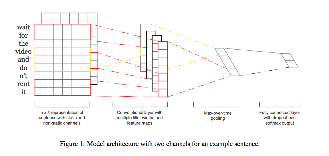
在本文中，构建的TextCNN网络结构如下图所示，只是简单的使用了几个网络结构进行处理。其中AdaptiveMaxPool是Pytorch提供的一个模块，它能够自动调整池化层的kernel大小，使得输出为指定的shape。

代码及结果

代码示意图如下：

class MyNet(nn.Module):    def __init__(self,embedding_size):        super(MyNet,self).__init__()        self.embedding = nn.Embedding.from_pretrained(embedding_weight,freeze=False)        self.conv = nn.Conv2d(1,256,(3,embedding_size)) # kernel_size 为(3,embedding_size)        self.adaptive_max_pool = nn.AdaptiveMaxPool1d(2)        self.fc = nn.Sequential(            nn.Linear(256*2,128),            nn.Dropout(0.6),            nn.ReLU(),            nn.Linear(128,2),           )        def forward(self,x): # (batch_size,seq_len)        x = self.embedding(x) #(batch_size,seq_len,embedding_size)        x = x.unsqueeze(1) # (batch_size,1,seq_len,embedding_size) ，因为CNN的input为(N,C,H,W)        x = self.conv(x) #(batch_size,256,seq_len-2,1)        x = x.squeeze(3) #(batch_size,256,seq_len-2)        x = F.relu(x)        x = self.adaptive_max_pool(x) #(batch_size,256,2)        x = torch.cat((x[:,:,0],x[:,:,1]),dim=1) #(batch_size,256*2)        output = self.fc(x)        return F.log_softmax(output,dim=1)        device = torch.device("cuda:0" if torch.cuda.is_available() else "cpu")my_net = MyNet(embedding_weight.shape[1]).to(device)

最终训练过程的ACC如下所示，当验证集的loss最小时，测试集的acc为\(84.28\%\)。

混淆矩阵：

TextCNN	positive	negative
positive	152	23
negative	47	159

LSTM网络

原理及网络结构

LSTM的网络结构如下所示，在本文中，只是简单的利用了LSTM的网络最后一个状态的输出\(h_n\)，然后将其输入到全连接层中，最后输出预测结果。

代码及结果

代码如下，在模型中，使用了两层的LSTM。同时，为了提高LSTM模型的训练效率， 使用pack_padded_sequence对padding之后的数据进行处理（使用参考：pack_padded_sequence 和 pad_packed_sequence - 知乎 (zhihu.com)）。

import torch.nn as nnimport torchimport torch.nn.functional as Fimport torch.optim as optimclass MyNet(nn.Module):    def __init__(self,embedding_size,hidden_size,num_layers=2):        super(MyNet,self).__init__()        self.embedding = nn.Embedding.from_pretrained(embedding_weight,freeze=False)         self.num_layers = num_layers        self.lstm = nn.LSTM(embedding_size,hidden_size,batch_first=True,bidirectional=True,num_layers=self.num_layers)        self.fc = nn.Sequential(            nn.BatchNorm1d(hidden_size),            nn.Linear(hidden_size,128),            nn.Dropout(0.6),            nn.ReLU(),            nn.Linear(128,2),           )        def forward(self,input,data_len):                input = self.embedding(input)        input = nn_utils.rnn.pack_padded_sequence(input,data_len,batch_first=True,enforce_sorted=False)        _,(h_n,c_n) = self.lstm(input) # h_n(num_layers*2,batch_size,hidden_size)        h_n = torch.permute(h_n,(1,0,2)) # h_n(batch_size,num_layers*2,hidden_size)        h_n = torch.sum(h_n,dim=1) # h_n (batch_size,hidden_size)        output = self.fc(h_n)        return F.log_softmax(output,dim=1)        device = torch.device("cuda:0" if torch.cuda.is_available() else "cpu")my_net = MyNet(embedding_weight.shape[1],512).to(device)

最终训练过程的ACC如下所示，当验证集的loss最小时，测试集的acc为\(81.57\%\)。

混淆矩阵：

LSTM	positive	negative
positive	140	21
negative	47	161

Attention-Based BiLSTM

原理及网络结构

在https://aclanthology.org/P16-2034.pdf论文中，Attention-Based BiLSTM算法的结构图如下所示：

Attention Layer的输入：

\[h_{i}=\left[\overrightarrow{h_{i}} \oplus \overleftarrow{h_{i}}\right]\]

设\(H\)是\(T\)个词经过BiLSTM得到的向量的集合：\(H = [h_1,h_2,\dots,h_T]\)。

Attention的计算，其中\(w\)便是需要训练的参数。

\[M = tanh(H)\\\alpha = softmax(w^TM)\]

Attention层的输出为：

\[r = H\alpha^T\]

代码及结果

下面的代码分别参考了两位博主的代码，被注释的参考了5，没被注释的参考了6。没注释的代码跑出来的效果更好一点（但是被注释的代码更加符合论文的流程）。

class MyNet(nn.Module):    def __init__(self,embedding_size,hidden_size,num_layers=1):        super(MyNet,self).__init__()        # 使用与训练好的词向量权重        self.embedding = nn.Embedding.from_pretrained(embedding_weight,freeze=False)         self.hidden_size = hidden_size        self.num_layers = num_layers        self.lstm = nn.LSTM(embedding_size,hidden_size,batch_first=True,bidirectional=True,num_layers=self.num_layers)                # self.w = nn.Parameter(torch.Tensor(hidden_size,1))        self.attention_w = nn.Sequential(            nn.Linear(hidden_size,hidden_size),            nn.Dropout(0.6),            nn.ReLU()        )        self.fc = nn.Sequential(            nn.BatchNorm1d(hidden_size),            nn.Linear(hidden_size,256),            nn.Dropout(0.6),            nn.ReLU(),            nn.Linear(256,2),        )            def attention_layer(self,lstm_output,lstm_h_n = None):        """            lstm_output：(batch_size,seq_len,hidden_size*2)            lstm_h_n：(num_layers*2,batch_size,hidden_size)        """        # H = lstm_output[:,:,:self.hidden_size] + lstm_output[:,:,self.hidden_size:] # (batch_size,seq_len,hidden_size)        # M = H # (batch_size,seq_len,hidden_size)        # # w        # lstm_h_n = lstm_h_n.permute(1,0,2) # (batch_size,num_layers*2,hidden_size)        # lstm_h_n = torch.sum(lstm_h_n,dim=1) # (batch_size,hidden_size)        # w = self.attention_w(lstm_h_n) # (batch_size,hidden_size)        # w = lstm_h_n.unsqueeze(dim=1) # (batch_size,1,hidden_size)        # # 生成alpha        # alpha = F.softmax(torch.bmm(w,M.permute(0,2,1)),dim=2) # (batch_size,1,seq_len)        # # 生成r        # r = torch.bmm(alpha,H) #(batch_size,1,hidden_size)        # r = r.squeeze(1)    #(batch_size,hidden_size)        # return r         lstm_h_n = lstm_h_n.permute(1,0,2) # (batch_size,num_layers*2,hidden_size)        lstm_h_n = torch.sum(lstm_h_n,dim=1) # (batch_size,hidden_size)        attention_w = self.attention_w(lstm_h_n) # (batch_size,hidden_size)        attention_w = attention_w.unsqueeze(dim=2) # (batch_size,hidden_size,1)        H = lstm_output[:,:,:self.hidden_size] + lstm_output[:,:,self.hidden_size:] # (batch_size,seq_len,hidden_size)                # alpha = F.softmax(torch.matmul(H,self.w),dim=1) #(batch_size,seq_len,1)        alpha = F.softmax(torch.matmul(H,attention_w),dim=1) #(batch_size,seq_len,1)        r = H * alpha # (batch_size,seq_len,hidden_size)        out = torch.relu(torch.sum(r,1)) #(batch_size,hidden_size)        return out        def forward(self,input,data_len=None):        input = self.embedding(input)        input = nn_utils.rnn.pack_padded_sequence(input,data_len,batch_first=True,enforce_sorted=False)        output,(h_n,c_n) = self.lstm(input) # output (batch_size,seq_len,hidden_size*2) h_n(num_layers*2,batch_size,hidden_size)        output,_ = nn_utils.rnn.pad_packed_sequence(output,batch_first=True)        output = self.attention_layer(output,h_n) #(batch_size,hidden_size)        output = self.fc(output) # (batch_size,2)        return F.log_softmax(output,dim=1)        device = torch.device("cuda:0" if torch.cuda.is_available() else "cpu")my_net = MyNet(embedding_weight.shape[1],512,num_layers=1).to(device)

最终训练过程的ACC如下所示，当验证集的loss最小时，测试集的acc为\(85.64\%\)。

混淆矩阵：

Attention-Based BiLSTM	positive	negative
positive	161	27
negative	26	155

总结

本文使用了3中模型对电影评论进行了分类。在实验中，发现TextCNN和Attention-Based BiLSTM模型的效果比较好。

尽管Attention-Based BiLSTM取得效果略好于TextCNN，但是其在训练的过程中需要耗费更多的时间，这是由LSTM的特性所决定的。

Reference

1. pack_padded_sequence 和 pad_packed_sequence - 知乎 (zhihu.com)

2. CNNs for Text Classification – Cezanne Camacho – Machine and deep learning educator.

3. AdaptiveMaxPool1d — PyTorch 1.11.0 documentation

4. https://aclanthology.org/P16-2034.pdf

5. xiaobaicxy/text-classification-BiLSTM-Attention-pytorch: 文本分类， 双向lstm + attention 算法 (github.com)

6. 文本分类算法之BiLSTM+Attention - 朴素贝叶斯 - 博客园 (cnblogs.com)